Python for AI: From Zero to First Model

Book 3 of 10 — AstolixGen Learning Series (Detailed Edition) · For researcher and publication students

---

About This Book

Python is the language nearly all modern AI research is written in. Every machine learning paper you read — every model you train, every dataset you clean, every graph you put in your publication — runs on Python and its ecosystem of libraries. This book takes you from a fresh Python install to training and evaluating your first machine learning model, with the habits that make your code reproducible and publication-ready.

Unlike generic Python tutorials, this book is written for you: a researcher or publication student (MS/PhD, early researcher). Every chapter ends with practical advice on how the topic connects to your thesis, your experiments, and your papers. You will write real code in every chapter, and you will finish with a complete mini-project you can document as a research artifact.

Learning objectives: - Install and configure Python, pip, virtual environments, and Jupyter notebooks for AI work - Write clean, working Python code using types, control flow, functions, and comprehensions - Use NumPy arrays, broadcasting, and vectorization for fast numerical computing - Load, inspect, and clean real datasets with Pandas - Create exploration and publication-quality plots with Matplotlib and Seaborn - Train, evaluate, and tune a classifier end to end with scikit-learn - Debug and profile machine learning code efficiently - Make experiments reproducible with random seeds, environment management, and dependency pinning - Structure a project so it grows from a notebook to a reusable codebase - Document code and results to the standard a paper or thesis expects

---

Learning Dashboard

Concept	Definition (one line)	Example	Use in research
Python	General-purpose, readable programming language used across AI research	model.fit(X_train, y_train)	Writing every experiment, script, and tool
pip	Python's package installer for adding libraries	pip install numpy	Installing research libraries (scikit-learn, pandas)
Virtual environment	An isolated Python setup so each project has its own packages	python -m venv ai-env	Keeping experiments reproducible and conflict-free
Jupyter notebook	Interactive document mixing code, output, and text	notebook.ipynb cell running analysis	Exploring data and drafting experiment narratives
Variable / type	Named storage with a data kind (int, float, str, list)	accuracy = 0.94	Storing metrics, parameters, results
List	Ordered, changeable collection of items	scores = [0.91, 0.93, 0.89]	Holding fold scores, predictions
Dictionary	Key-value mapping for named lookups	{"model": "SVM", "acc": 0.93}	Configs, results logs, metadata
Function	Reusable named block of code with inputs and outputs	def train_model(X, y):	Repeating experiment steps reliably
List comprehension	One-line expression building a list	[x**2 for x in range(10)]	Clean, fast data transformations
NumPy array (ndarray)	Fast, fixed-type N-dimensional array for math	np.array([[1, 2], [3, 4]])	Storing features, images, weights
Broadcasting	NumPy rule that aligns different-shaped arrays in math	arr + 5 adds 5 to every element	Normalizing data without loops
Vectorization	Replacing Python loops with array operations	np.mean(arr, axis=0) vs a loop	10–100x faster experiment code
Pandas DataFrame	Table with labeled rows and columns	pd.read_csv("data.csv")	Loading and cleaning real datasets
Pandas Series	One labeled column of a DataFrame	df["label"]	Feature/target extraction
Missing values	Gaps in data (NaN) that must be handled	df.fillna(df.mean())	Cleaning datasets before training
Matplotlib	Core plotting library for Python	plt.plot(x, y)	Line plots, figure control
Seaborn	High-level statistical plots on top of Matplotlib	sns.heatmap(cm)	Confusion matrices, distributions
Scikit-learn	The standard ML library: models, metrics, pipelines	LogisticRegression().fit(X, y)	Training and evaluating classifiers
Feature	Input variable the model learns from	df[["age", "bp"]]	Model inputs in every experiment
Label (target)	The answer the model must predict	df["disease"]	Supervised learning ground truth
Train/test split	Dividing data into learning and held-out evaluation sets	train_test_split(X, y, test_size=0.2)	Honest, credible model evaluation
Classifier	Model that predicts a category label	SVC(), RandomForestClassifier()	Baseline models for papers
Cross-validation	Rotating train/test splits to estimate performance robustly	cross_val_score(model, X, y, cv=5)	Reliable results for publication tables
Hyperparameter	Setting chosen by you, not learned by the model	max_depth=5	Tuning reported in methodology sections
Overfitting	Model memorizes training data, fails on new data	Train acc 99%, test acc 61%	The main failure mode to diagnose
Random seed	Fixed starting point for randomness	random_state=42	Reproducible splits and training
Reproducibility	Anyone can rerun your code and get the same result	Seed + pinned versions + documented env	Required standard for published research
Dependency pinning	Recording exact library versions used	numpy==1.26.4 in requirements.txt	Rerunning code months later
Debugging	Finding and fixing why code behaves wrongly	Traceback reading, prints, breakpoints	Fixing shape mismatches, NaNs, crashes
Profiling	Measuring where code spends time	%timeit, cProfile	Speeding up slow experiments

Roadmap — how the chapters connect: Chapter 1 explains why Python is the right bet, then Chapters 2–3 give you a working setup and the language basics. Chapters 4–6 build your three daily tools — NumPy (numbers), Pandas (tables), Matplotlib/Seaborn (plots) — the same stack almost every published ML experiment uses [1], [2]. Chapter 7 is the payoff: your first trained model with scikit-learn, with Chapters 8–9 covering the real-world skills of dataset handling, debugging, and profiling. Chapters 10–11 teach you the professional habits (reproducibility, project structure) that separate a student script from publishable research code. Chapter 12 ties it all together in a complete mini-project documented like a paper artifact.

---

Chapter 1: Why Python Dominates AI Research

If you look at the code behind any recent machine learning paper, it is almost certainly Python. This is not an accident, and it is not just fashion. Python won AI research for concrete, practical reasons that matter directly to you as a student: it makes experiments fast to write, fast to run, and fast to share.

The practical reasons Python won

1. Readability speeds up research. Research code is read far more often than it is written — by you next month, by your supervisor, by reviewers. Python reads close to plain English. Compare what it takes to compute the average of a column: in Python, np.mean(scores). The clarity means fewer bugs and faster iteration. When you are testing ten ideas a week, the language that gets out of your way wins.

2. The library ecosystem does the heavy lifting. You never write a neural network or a classifier from scratch. NumPy handles arrays, Pandas handles tables, scikit-learn handles classical models [1], and PyTorch [3] and TensorFlow [4] handle deep learning. These libraries are written by large communities, tested by millions of users, and optimized in fast C/C++ code underneath. You write short, readable Python; the heavy math runs at machine speed. This is the single biggest reason a student can reproduce a paper's experiment in an afternoon.

3. Reproducibility is built into the culture. The Python AI community expects code, data, and exact environments to be shared. Standard tools — requirements.txt, virtual environments, random seeds, notebooks — are exactly what journals now ask for when they say "make your work reproducible." Learning Python is learning the reproducibility workflow at the same time.

4. Notebooks match how research actually happens. Research is exploratory: try something, look at the result, adjust. Jupyter notebooks let you run code in small steps, see tables and plots right next to the code, and write explanations between cells. The exploratory loop in a notebook is the natural home of early-stage research.

5. Everyone you need is already here. Your supervisor's students, the paper authors whose code you download, Stack Overflow answers, dataset loaders, university courses — all speak Python. Choosing Python means every question you ask has an answer somewhere, and every tool you need already exists.

What Python is NOT (honest limitations)

Python is slow at raw number crunching in pure form — a Python loop over a million numbers can be a hundred times slower than the same loop in C. The ecosystem solves this: NumPy, Pandas, and scikit-learn push the heavy work into compiled code, so your Python is just the conductor, not the orchestra. You will learn this pattern (called vectorization) in Chapter 4, and it is one of the most valuable skills in this book.

Python also has quirks — dynamic typing means a variable can silently change type and cause a confusing error later, and the famous "dependency hell" (library versions conflicting) is real. Chapters 2 and 10 teach you the standard defenses: virtual environments, pinning versions, and writing small testable functions.

The AI Python stack, top to bottom

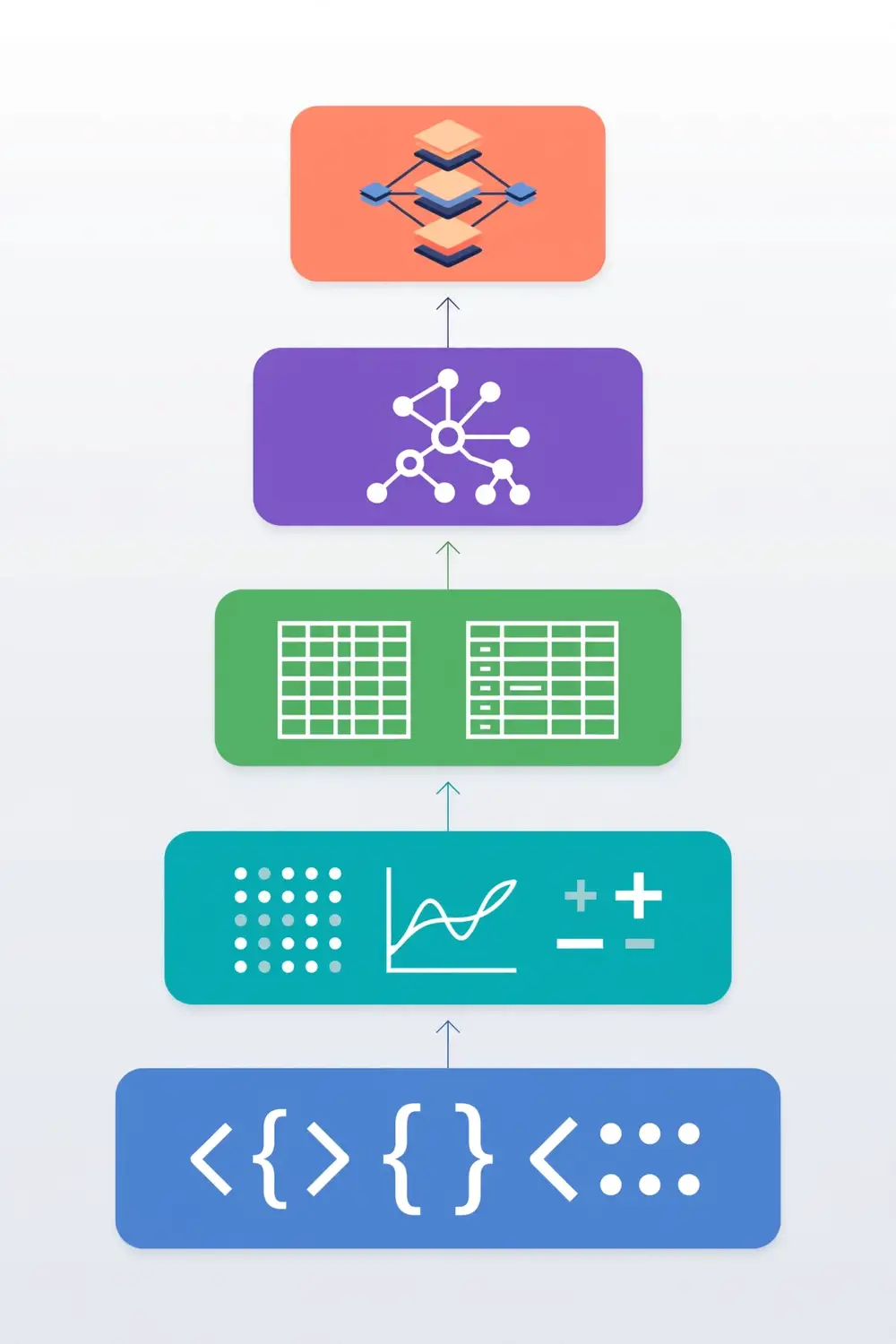
You can think of the ecosystem as layers, each built on the one below:

• Layer 1 — Python itself. The language: syntax, data structures, functions.
• Layer 2 — NumPy and Pandas. Fast arrays and data tables. Almost every experiment touches these.
• Layer 3 — scikit-learn. Classical machine learning: classifiers, regressors, clustering, evaluation metrics [1].
• Layer 4 — PyTorch and TensorFlow. Deep learning: neural networks, GPUs [3], [4].

Books 5 and 6 of this series will take you into deep learning. This book makes you strong in Layers 1–3, which is exactly where most student publications live: data loading, cleaning, classical models, evaluation, and clear plots.

Worked example: the whole stack in 15 lines

Here is a complete machine learning experiment in Python. Do not worry if the details are unfamiliar — every piece is explained in later chapters. The point is how little code it takes:

import pandas as pd                      # Layer 2: tables
from sklearn.model_selection import train_test_split
from sklearn.ensemble import RandomForestClassifier
from sklearn.metrics import accuracy_score

df = pd.read_csv("patients.csv")         # load data
X = df[["age", "blood_pressure", "cholesterol"]]
y = df["disease"]                        # features and label

X_train, X_test, y_train, y_test = train_test_split(
    X, y, test_size=0.2, random_state=42)

model = RandomForestClassifier(random_state=42)
model.fit(X_train, y_train)              # train
preds = model.predict(X_test)            # predict

print("Accuracy:", accuracy_score(y_test, preds))

Fifteen lines: load data, split it, train a model, evaluate it. In older languages this same experiment could take hundreds of lines. That compression is why Python dominates — and why you can realistically go from zero to a publishable experiment in weeks, not months.

Python vs. the alternatives — an honest comparison

You may hear about other languages. Here is the short, honest version:

• R — excellent for statistics and beloved in some social-science and biostatistics departments. But most new machine learning methods are published in Python first, and the deep learning ecosystem barely exists in R.
• MATLAB — still common in engineering faculties, with good toolboxes. Downsides: expensive licenses, and almost nobody publishes reproducible ML code in it anymore.
• Julia — fast, elegant, and designed for scientific computing. But the community is small, Stack Overflow answers are scarce, and production tooling is thin.

None of these is "bad." But research is a team sport played with shared tools, and Python is where the team is. When a paper releases code (increasingly expected), it is Python. When a dataset publishes a loader, it is Python. When you get stuck at 2 a.m., the answer exists for Python.

What "knowing Python for AI" actually means

It does not mean memorizing syntax or passing a quiz on language trivia. It means you can do six things reliably:

1. Load data from a file into a usable structure.
2. Clean and explore it (Chapters 5–6).
3. Train a model and evaluate it honestly (Chapter 7).
4. Make the whole thing rerunnable by someone else (Chapter 10).
5. Organize it so it grows (Chapter 11).
6. Explain what you did in writing (Chapter 12).

Notice that only a small part of that list is "the Python language." Most of it is workflow — and workflow is exactly what this book teaches. A student who can do those six things is more useful in a lab than one who knows every language feature but cannot finish an experiment.

A note on AI-assisted coding

Tools that write code for you are now everywhere, and you should use them — but as an accelerator, not a replacement. They are excellent at boilerplate ("write a function that loads a CSV and prints summary stats") and dangerous at the parts that require judgment (choosing metrics, spotting leakage). The rule: never run generated code you could not explain line by line. This book gives you the understanding that makes AI assistants safe to use.

Python versions: why 3.11, and why it matters

Python releases a new minor version yearly (3.10, 3.11, 3.12...), and AI libraries need months to catch up — compiled packages like NumPy must be rebuilt for each version. That is why this book recommends 3.11: new enough for modern features and speed improvements (3.11 is roughly 25% faster than 3.10), old enough that every library you need supports it. Two rules: never chase the newest release for research work, and always record the exact version (Chapter 10). A one-line version difference has broken more student experiments than any bug.

Getting help effectively: the minimal reproducible example

You will get stuck — everyone does. When you ask for help (supervisor, forum, AI assistant), include a minimal reproducible example: the smallest complete code that shows the problem, plus the full error message:

# Good help request: 6 lines, runs anywhere, error included
import numpy as np
from sklearn.linear_model import LogisticRegression
X = np.array([1, 2, 3])          # 1-D by mistake
model = LogisticRegression().fit(X, [0, 1, 0])
# ValueError: Expected 2D array, got 1D array instead

Preparing the example solves half of all problems by itself — shrinking the code isolates the bug. And responders answer good examples in minutes while ignoring "my code doesn't work" with no details.

For your research: When your supervisor or a reviewer asks "why Python?", the honest answer is: it is the language of the field's shared infrastructure. Choosing it means you inherit the libraries, the datasets loaders, the pretrained models, and the community that produced the papers you cite. Note this choice in your thesis methodology section — reviewers expect it, and one sentence ("All experiments were implemented in Python 3.11 using scikit-learn 1.3 [1]...") signals you follow standard practice.

Key takeaways - Python dominates AI because of readability, the library ecosystem, reproducibility culture, notebooks, and community size. - The stack is layered: Python → NumPy/Pandas → scikit-learn → PyTorch/TensorFlow. - Python is slow in raw loops; the ecosystem fixes this with vectorized compiled code underneath. - Most student papers live in Layers 1–3: data, classical models, evaluation, plots — exactly this book's territory.

---

Chapter 2: Setup — Python, pip, Virtual Environments, and Jupyter

A correct setup saves you from the most common beginner disaster: code that works on your laptop today and breaks everywhere else tomorrow. Spend one careful hour here and it pays back for your entire degree.

Installing Python

Download Python 3.11 or newer from python.org (avoid 3.13+ for now — some AI libraries lag behind new releases). During installation on Windows, check the box "Add python.exe to PATH" — this is the step most beginners miss, and without it the terminal cannot find Python.

Verify with:

python --version
# Python 3.11.9

If that prints a version, you are set. On some systems the command is python3 instead of python; pick whichever works and use it consistently.

pip: installing libraries

pip is Python's package installer, and it comes with Python. Installing a library is one command:

pip install numpy pandas matplotlib seaborn scikit-learn jupyter

This installs the core AI stack: NumPy (arrays), Pandas (tables), Matplotlib and Seaborn (plots), scikit-learn (models) [1], and Jupyter (notebooks). Check an install worked:

python -c "import sklearn; print(sklearn.__version__)"
# 1.3.2

The -c flag runs a one-line Python program — handy for quick checks.

Practical tip: keep a requirements.txt file listing what you installed. Chapter 10 will show you how to generate one automatically (pip freeze), but even a hand-written list today saves confusion later.

Virtual environments: one project, one sandbox

Here is the problem virtual environments solve. Project A needs scikit-learn 1.3. Project B needs scikit-learn 1.1 (an older paper's code). Installed globally, they conflict and one project breaks. A virtual environment is a private Python sandbox per project — each has its own packages, and they never fight.

Create and activate one:

# Create (do this once per project)
python -m venv ai-env

# Activate — Windows
ai-env\Scripts\activate

# Activate — macOS/Linux
source ai-env/bin/activate

Your terminal prompt changes to show (ai-env) at the front — that is your confirmation. Now pip install goes into the sandbox only. When you are done, deactivate exits it.

Rule of thumb: one virtual environment per project, created in the project folder. Name it .venv or ai-env and never commit it to Git (add it to .gitignore). This single habit prevents the majority of "it worked on my machine" failures.

Jupyter notebooks: your lab notebook

Install Jupyter (inside your virtual environment), then launch:

pip install notebook
jupyter notebook

A browser tab opens showing your files. Create a new notebook (.ipynb) and you get cells — boxes where you type code and press Shift+Enter to run. Output, including tables and plots, appears directly under the cell. Between code cells you can add Markdown cells for headings and explanations (double-click a cell and choose Markdown from the dropdown, or press Esc then M).

The workflow that makes notebooks powerful for research:

1. Load data in one cell, inspect it in the next.
2. Try a plot, see it immediately, adjust.
3. Write a paragraph of what you observed — this becomes your paper's results narrative later.
4. When an experiment works, the notebook is already half of your documentation.

Two honest warnings about notebooks. First, cells can be run in any order, which means the notebook on screen may not match a top-to-bottom run — always do Kernel → Restart & Run All before trusting results. Second, notebooks are for exploration, not for final reusable code — Chapter 11 shows when and how to graduate working code into plain .py scripts.

Worked example: verify your whole setup in one notebook

Create a notebook and run these cells in order. If every cell runs without errors, your environment is ready:

# Cell 1: check the core libraries
import numpy as np
import pandas as pd
import matplotlib.pyplot as plt
import sklearn
print("numpy", np.__version__)
print("pandas", pd.__version__)
print("sklearn", sklearn.__version__)

# Cell 2: make a tiny dataset and plot it
data = {"x": [1, 2, 3, 4, 5], "y": [2, 4, 5, 4, 5]}
df = pd.DataFrame(data)
df.plot(x="x", y="y", kind="scatter")
plt.title("Setup check: my first plot")
plt.show()

# Cell 3: train a toy model
from sklearn.linear_model import LinearRegression
model = LinearRegression()
model.fit(df[["x"]], df["y"])
print("Prediction for x=6:", model.predict([[6]])[0])

Three cells: libraries verified, a plot rendered, a model trained. Save this notebook as setup_check.ipynb in your project folder — rerunning it is the fastest way to check a new machine or a fresh environment.

Anaconda vs. plain Python + pip

You will see two recommended setups and wonder which to pick:

• Anaconda / Miniconda — a distribution bundling Python with 250+ scientific packages and its own environment manager (conda). One big installer, fewer compilation headaches on Windows, and conda install sometimes succeeds where pip struggles with tricky packages.
• Plain Python + pip + venv — lighter, faster, and what this book uses. You install exactly what you need.

Either works. Start with plain Python; if a package repeatedly fails to install (common with some scientific libraries on Windows), try Miniconda for that project. Do not mix both managers in one environment — pick one per project and stick with it.

Common setup problems and fixes

Almost every beginner hits one of these. None of them means you did something wrong:

Symptom	Likely cause	Fix
'python' is not recognized	Missed the "Add to PATH" checkbox	Reinstall with the box checked, or use the py launcher (py --version)
pip install fails with C++ / compiler errors	Package needs compilation	On Windows, install Microsoft C++ Build Tools; or use conda for that package
Jupyter kernel dies immediately	Notebook using a different Python than your venv	In the venv: pip install ipykernel, then select the venv kernel in the notebook
import sklearn works in terminal but not notebook	Same as above — kernel/environment mismatch	Check sys.executable in both; they must match
Two Pythons fighting (python vs python3)	Multiple installs	where python (Windows) / which -a python3 (macOS/Linux) to see them; use the full path or virtual environments to disambiguate

The golden diagnostic: when imports behave strangely, run this in the exact place the code runs (terminal or notebook cell):

import sys
print(sys.executable)   # which Python is this, exactly?

Nine times out of ten, the answer is "not the one you thought," and the fix is activating the right environment.

Keeping your setup healthy over time

• Upgrade pip occasionally: pip install --upgrade pip.
• Do not install every interesting package into one environment — that is how conflicts start. New project, new venv.
• Once a month, delete environments for finished or abandoned projects (rm -rf ai-env after deactivating). They are cheap to recreate from requirements.txt (Chapter 10).

Your first-week routine

Setup is done — now build the habit. A routine that works for busy students:

• Day 1–2: Run every snippet in Chapters 3–4 in a notebook. Type them; do not copy-paste. Typing builds muscle memory.
• Day 3–4: Load a real CSV (any you can find) and run the Chapter 5 inspection ritual on it.
• Day 5: Train the Chapter 7 classifier on the breast cancer dataset. Change one hyperparameter and observe the effect.
• Day 6–7: Break something deliberately — delete a random_state, fit the scaler on all data — and watch the numbers change. Understanding why they change is the lesson.

Thirty focused minutes daily beats a monthly marathon. Research coding is a practice, like lab technique: regular, deliberate, and recorded in your notebook.

JupyterLab vs. classic Notebook

pip install notebook gives the classic interface; JupyterLab (pip install jupyterlab, run jupyter lab) is its modern successor — tabs, a file browser, a visual debugger, and a better text editor in one window. Either is fine for this book; JupyterLab is the better long-term home as your projects grow. VS Code with the Python and Jupyter extensions is a popular third option that many labs standardize on.

For your research: Your thesis or paper methodology should name your exact environment: Python version, key library versions, and operating system. Create this record the day you start, not the day you submit. A simple environment.txt with the output of python --version and pip freeze is enough. Reviewers increasingly ask for it, and reconstructing it months later from memory is unreliable.

Key takeaways - Install Python 3.11+, verify with python --version, install libraries with pip. - One virtual environment per project (python -m venv ai-env) — never install research packages globally. - Jupyter notebooks are your exploratory lab: run cells, see output, write explanations alongside. - Always Restart & Run All before trusting a notebook; notebooks are for exploration, scripts are for reuse. - Record your environment from day one — future-you (and your reviewers) will thank you.

---

Chapter 3: Python Essentials Refresher

This chapter covers the 20% of Python you will use 80% of the time in AI work. If you have programmed before, skim fast and do the worked example. If Python is new to you, type every snippet into a notebook and run it — reading code teaches little; running it teaches a lot.

Variables and types

A variable is a named box holding a value. Python figures out the type automatically:

name = "Asif"          # str — text
epoch = 10             # int — whole number
accuracy = 0.942       # float — decimal number
done = True            # bool — True/False

Check a type with type(accuracy) → <class 'float'>. The key types in AI code are int, float, str, list, dict, and later ndarray (NumPy) and DataFrame (Pandas).

Dynamic typing gotcha: a variable can be reassigned to a different type (x = 5 then x = "five"), and Python will not warn you. In long experiment scripts this causes confusing errors far from the mistake. The defense: keep variable names meaningful (test_accuracy, not x) and re-run cells top to bottom.

Collections: lists, tuples, dictionaries

Lists hold ordered items and can be changed:

scores = [0.91, 0.87, 0.93]   # three cross-validation scores
scores.append(0.89)            # add one
print(scores[0])               # first item: 0.91 (indexing starts at 0)
print(scores[-1])              # last item: 0.89
print(scores[0:2])             # slice: [0.91, 0.87]

Tuples are like lists but unchangeable — used for fixed records:

image_shape = (256, 256, 3)    # height, width, color channels

Dictionaries map keys to values — the workhorse for configs and results:

config = {"model": "random_forest", "max_depth": 5, "n_estimators": 100}
print(config["model"])         # random_forest
config["accuracy"] = 0.93      # add a new key

You will log experiment results as dictionaries and configs as dictionaries throughout your research career.

Control flow: if, for, while

# if: make decisions
if accuracy >= 0.90:
    print("Good enough to report")
elif accuracy >= 0.80:
    print("Needs tuning")
else:
    print("Try a different approach")

# for: repeat over a collection
for depth in [3, 5, 10]:
    model = RandomForestClassifier(max_depth=depth)
    model.fit(X_train, y_train)
    print(depth, model.score(X_test, y_test))

# while: repeat until a condition changes (use sparingly)
epoch = 0
while epoch < 3:
    print("training epoch", epoch)
    epoch += 1

The for loop over a list of hyperparameter values is the simplest form of hyperparameter search — you will write this pattern constantly.

Functions: name it, reuse it

A function packages logic with a name, inputs, and an output:

def evaluate(model, X_test, y_test):
    """Return accuracy of a fitted model on test data."""
    preds = model.predict(X_test)
    return (preds == y_test).mean()

acc = evaluate(model, X_test, y_test)
print(f"Test accuracy: {acc:.3f}")   # f-string formatting: 0.933

Three habits that make functions research-grade:

1. One job per function — load_data(), train(), evaluate(), not one giant do_everything().
2. A docstring (the """...""" line) saying what it returns. Future-you will forget; the docstring remembers.
3. Return values instead of printing — returned values can be logged, compared, and put in tables; printed values vanish.

Comprehensions: clean one-line transformations

A list comprehension builds a list in one readable line:

# The long way
cleaned = []
for s in scores:
    cleaned.append(round(s, 2))

# The comprehension way
cleaned = [round(s, 2) for s in scores]

# With a condition
good = [s for s in scores if s >= 0.90]

Dictionary comprehensions work the same way: {m: evaluate(m, X_test, y_test) for m in models} builds a name→accuracy map in one line. Comprehensions are not just style — they are faster than explicit loops and they are the idiom reviewers and collaborators expect.

Worked example: a tiny experiment harness

This example combines everything — it trains three models, evaluates each, and reports the winner, the pattern you will reuse in every comparative study:

from sklearn.datasets import load_iris
from sklearn.model_selection import train_test_split
from sklearn.linear_model import LogisticRegression
from sklearn.svm import SVC
from sklearn.ensemble import RandomForestClassifier

def run_comparison(models, X_train, X_test, y_train, y_test):
    """Train each model and return {name: accuracy}."""
    results = {}
    for name, model in models.items():
        model.fit(X_train, y_train)
        results[name] = round(model.score(X_test, y_test), 3)
    return results

X, y = load_iris(return_X_y=True)
X_train, X_test, y_train, y_test = train_test_split(
    X, y, test_size=0.2, random_state=42)

models = {
    "logistic_regression": LogisticRegression(max_iter=200),
    "svm": SVC(),
    "random_forest": RandomForestClassifier(random_state=42),
}

results = run_comparison(models, X_train, X_test, y_train, y_test)
for name, acc in sorted(results.items(), key=lambda kv: kv[1], reverse=True):
    print(f"{name:20s} {acc:.3f}")

best = max(results, key=results.get)
print("Winner:", best)

Expected output (your numbers may differ slightly by version):

random_forest        1.000
logistic_regression  1.000
svm                  0.967
Winner: random_forest

On the small Iris dataset, simple models often tie — and that is itself a research lesson: always report all compared models, not just the winner, because the comparison table is what a paper's results section is built from.

f-strings: reporting numbers cleanly

You will print metrics hundreds of times. f-strings (formatted string literals) are the clean way:

acc = 0.93347
print(f"Accuracy: {acc:.3f}")        # Accuracy: 0.933  (3 decimals)
print(f"Accuracy: {acc:.1%}")        # Accuracy: 93.3%  (percentage)
print(f"Samples: {12500:,}")         # Samples: 12,500  (thousands separator)
print(f"Model: {name:20s} {acc:.3f}")# padded column — neat tables in the terminal

Format specs worth memorizing: :.3f (decimals), :.1% (percent), :, (thousands), :20s (padded text). Clean console output becomes your lab notebook's first draft.

Gotchas that bite researchers

1. Mutable default arguments. This is Python's most famous trap:

def add_result(score, results=[]):   # DANGER: the list persists between calls!
    results.append(score)
    return results

Call it twice and the second call sees the first call's scores. The fix:

def add_result(score, results=None): # safe pattern
    if results is None:
        results = []
    results.append(score)
    return results

2. Float comparison. Never compare floats with == — tiny representation errors make 0.1 + 0.2 == 0.3 false. Use a tolerance:

abs(a - b) < 1e-9        # or
import math; math.isclose(a, b)

This matters when you assert that two runs produced "the same" metric.

3. Notebook variable ghosts. In notebooks, a variable set in a cell you later deleted still exists in the kernel. If results look impossibly good, restart the kernel and run all cells — the ghost disappears and the truth appears.

4. is vs ==. Use == for value comparison (if acc == best:). Use is only for None (if x is None:) — a convention the whole ecosystem follows.

Reading error messages like a researcher

You will see three error types constantly — learn their meaning once:

• NameError: name 'df' is not defined — you used a variable before creating it (or the cell that creates it did not run).
• TypeError: unsupported operand — wrong types mixed, e.g., adding a string to a number; check type() of each piece.
• KeyError: 'age' — dictionary/DataFrame has no such key; check spelling and df.columns.

Each error names the line and the values involved. Read it literally — it is almost always telling the truth.

Iteration helpers: enumerate, zip, unpacking

Three small tools that make loops cleaner — you will see them in every codebase you read:

models = ["lr", "svm", "rf"]
scores = [0.91, 0.87, 0.93]

for i, name in enumerate(models):       # index + value together
    print(i, name)

for name, score in zip(models, scores): # walk two lists in parallel
    print(f"{name}: {score:.2f}")

best_name, best_score = "rf", 0.93      # unpacking: one line, two variables
first, *rest = scores                   # first=0.91, rest=[0.87, 0.93]

zip is how you pair model names with their scores for reporting; enumerate replaces manual counter variables. Small, but they remove entire categories of off-by-one mistakes.

Comprehensions vs. map/filter

Older code uses map and filter; modern Python prefers comprehensions — they read better and the community standard is clear:

# Equivalent, but the comprehension is the idiom reviewers expect
squared = [x**2 for x in range(10)]          # prefer this
squared = list(map(lambda x: x**2, range(10)))  # not this

Nested comprehensions flatten grids and matrices: [v for row in matrix for v in row] turns a 2-D list into 1-D. Read it as nested loops, left to right.

For your research: Every paper's results section is a comparison table: rows are methods, columns are metrics. The run_comparison pattern above is that table in code form. Build this habit now: never evaluate one model in isolation — always evaluate a small set including at least one simple baseline (logistic regression is the classic). Reviewers distrust a new method that was never compared against a simple alternative.

Key takeaways - Master variables, lists, dicts, if/for, functions, and comprehensions — that is most of daily AI coding. - Dictionaries are your config and results-log format; functions should do one job and return values. - The train-several-models-and-compare pattern is the code behind every results table you will publish.

---

Chapter 4: NumPy — Numerical Computing Foundations

NumPy gives Python its number-crunching muscle. Its central object, the ndarray (N-dimensional array), stores data in a compact, fixed-type block of memory and performs math in compiled C code. Datasets, images, model weights, and predictions are all ndarrays underneath. If Pandas is the table you look at, NumPy is the engine room below it.

Creating and inspecting arrays

import numpy as np

a = np.array([1, 2, 3, 4])              # 1-D array (a vector)
b = np.array([[1, 2], [3, 4]])          # 2-D array (a matrix)
c = np.zeros((3, 4))                    # 3x4 array of zeros
d = np.ones((2, 2))                     # 2x2 array of ones
e = np.arange(0, 10, 2)                 # [0 2 4 6 8]
f = np.linspace(0, 1, 5)                # 5 evenly spaced values 0..1
g = np.random.rand(3, 3)                # 3x3 random values in [0, 1)

Every array has three vital attributes — learn to print them when confused:

print(b.shape)    # (2, 2)  — dimensions
print(b.ndim)     # 2       — number of dimensions
print(b.dtype)    # int64   — element type (all elements share one type)

The shape is the single most important debugging fact in ML code. Most errors you will meet are shape mismatches ("expected (100, 5), got (100,)"). Print shapes early and often.

Indexing and slicing

m = np.array([[1, 2, 3],
              [4, 5, 6],
              [7, 8, 9]])

print(m[0, 1])      # 2 — row 0, column 1
print(m[:, 1])      # [2 5 8] — all rows, column 1
print(m[1, :])      # [4 5 6] — row 1, all columns
print(m[0:2, 1:3])  # [[2 3] [5 6]] — sub-block
print(m[m > 5])     # [6 7 8 9] — boolean mask: elements where condition holds

Boolean masks (m[m > 5]) are how you filter data without loops — "give me all samples where the label is 1" is X[y == 1]. You will use this constantly when analyzing errors ("show me the images the model got wrong").

Vectorization: never loop when you can compute

A vectorized operation applies to the whole array at once, in compiled code:

# Slow: Python loop (avoid for large data)
result = []
for x in a:
    result.append(x ** 2)

# Fast: vectorized (do this)
result = a ** 2

The difference is not subtle — on a million elements, the loop can take a second while the vectorized version takes milliseconds. Rule: if you find yourself writing for over array elements to do math, stop and look for the NumPy function (np.mean, np.sum, np.max, np.dot, ...). Aggregation functions take an axis argument: np.mean(m, axis=0) averages down each column, axis=1 across each row.

Broadcasting: arithmetic on mismatched shapes

Broadcasting is NumPy's rule for combining arrays of different shapes: the smaller array is conceptually "stretched" to match. The classic use is normalization — subtract the mean of each column from every row:

data = np.array([[10., 20.],
                 [30., 40.],
                 [50., 60.]])

col_mean = data.mean(axis=0)     # [30. 40.] — shape (2,)
centered = data - col_mean       # broadcasts: subtracts from each row
print(centered)
# [[-20. -20.]
#  [  0.   0.]
#  [ 20.  20.]]

Broadcasting rules in one sentence: dimensions are aligned from the right, and a dimension of size 1 (or a missing dimension) stretches to match. When broadcasting fails, NumPy raises a clear error — read it, print the shapes, and you will see the fix.

Reshaping and stacking

v = np.arange(6)            # [0 1 2 3 4 5]
print(v.reshape(2, 3))      # 2 rows, 3 cols
print(v.reshape(-1, 2))     # -1 means "figure it out": 3 rows, 2 cols

flat = m.flatten()          # 2-D -> 1-D (images become feature vectors this way)
combo = np.vstack([a, a])   # stack vertically

reshape(-1, ...) is the idiom for "I know the columns, compute the rows." Flattening a 28×28 image to 784 numbers is exactly img.reshape(-1) — the first step of feeding images to a classical classifier.

Worked example: normalize a dataset and measure the speedup

Feature scaling (making columns comparable) is required by many models [2], and this example shows vectorization, broadcasting, and a timing comparison in one script:

import numpy as np
import time

rng = np.random.default_rng(42)
X = rng.normal(loc=50, scale=15, size=(20000, 10))  # 20k samples, 10 features

# Vectorized standardization: (x - mean) / std, per column
means = X.mean(axis=0)
stds = X.std(axis=0)
X_scaled = (X - means) / stds          # broadcasting does the work

print("Column means after scaling:", X_scaled.mean(axis=0).round(6))
# all ~0.0 — each feature now centered at zero

# Speed comparison: vectorized vs Python loop
t0 = time.perf_counter()
_ = (X - means) / stds
t_vec = time.perf_counter() - t0

t0 = time.perf_counter()
out = np.empty_like(X)
for i in range(X.shape[0]):
    for j in range(X.shape[1]):
        out[i, j] = (X[i, j] - means[j]) / stds[j]
t_loop = time.perf_counter() - t0

print(f"Vectorized: {t_vec*1000:.1f} ms | Loop: {t_loop*1000:.1f} ms "
      f"| Speedup: {t_loop/t_vec:.0f}x")

Typical output: Vectorized: 1.2 ms | Loop: 380.4 ms | Speedup: 317x. That gap is why vectorization is non-negotiable: on real datasets, loop-based preprocessing turns minutes into hours.

Lists vs. arrays: why the difference matters

A Python list is a collection of objects — each number carries type information and overhead (about 28 bytes per float). A NumPy array stores raw numbers packed together (8 bytes per float64) with one shared type. Consequences:

• Memory: a million floats as a list uses ~36 MB; as an array, ~8 MB. Datasets that fit comfortably in arrays can exhaust memory as lists.
• Speed: list math runs in Python (slow, one element at a time); array math runs in compiled C (fast, all at once) — the 300x gap you measured in the worked example.
• Expressiveness: data[data > threshold] has no list equivalent in one line.

The rule is simple: the moment data becomes numeric and sizable, it becomes an array. Lists remain for mixed or small collections (file names, model names, config values).

Random numbers the modern way

Old tutorials use np.random.seed() + np.random.rand(). The modern, recommended API uses a Generator object, which gives independent, reproducible streams:

rng = np.random.default_rng(42)   # seed once
a = rng.normal(0, 1, size=(100, 5))# 100x5 from a standard normal distribution
b = rng.integers(0, 10, size=50)  # 50 random integers in [0, 10)
c = rng.choice(["a", "b", "c"], size=20)  # random sampling from options

Use default_rng(SEED) in your own code (you saw it in the worked example). It is also what makes synthetic datasets for testing — like Chapter 12's capstone data — reproducible.

NumPy functions you will reach for weekly

Keep this list handy; each replaces a loop you might otherwise write:

np.mean(X, axis=0)      # column means (feature averages)
np.std(X, axis=0)       # column standard deviations
np.min(X), np.max(X)    # range checks — catch bad data fast
np.argmin(errors)       # index of the best model in a list of scores
np.unique(y)            # sorted unique values — instant class inventory
np.bincount(y)          # count of each integer label — class balance in one call
np.concatenate([a, b])  # join arrays
np.dot(A, B)  # or: A @ B   # matrix multiplication — the heart of ML math
np.linalg.norm(v)       # vector length — used in distance-based methods
np.percentile(X, 95)    # 95th percentile — robust outlier thresholds
np.where(X > 0, 1, 0)   # vectorized if/else — binarize in one line
np.isnan(X).any()       # the NaN check from Chapter 9

np.unique and np.bincount deserve emphasis: "what classes exist and how many of each?" is a question you ask of every dataset, and these answer it in one line.

Views vs. copies: NumPy's sneakiest gotcha

Slicing an array does not copy it — it creates a view sharing the same memory. Modifying the view modifies the original:

a = np.arange(5)        # [0 1 2 3 4]
b = a[1:4]              # view, not a copy!
b[0] = 99
print(a)                # [0 99 2 3 4] — the original changed!

This is a feature (views are free — no memory copied, which matters for large datasets), but it surprises everyone once. When you need independence, copy explicitly: b = a[1:4].copy(). Boolean-mask indexing (a[a > 2]) does return a copy — the inconsistency is historical, so when in doubt, .copy() and move on.

Thinking in axes

axis=0 means "down the rows" (collapsing rows, one result per column); axis=1 means "across the columns" (one result per row). The mnemonic: the axis number is the dimension that disappears:

m = np.array([[1, 2, 3],
              [4, 5, 6]])
print(m.mean(axis=0))   # [2.5 3.5 4.5] — one mean per column (rows collapsed)
print(m.mean(axis=1))   # [2. 5.]       — one mean per row (columns collapsed)

For a dataset shaped (samples, features), axis=0 gives per-feature statistics — the direction you aggregate in 90% of preprocessing. Getting axes wrong silently produces plausible-looking wrong numbers, so verify with a tiny example like the one above whenever you are unsure.

For your research: Reviewers will not ask "did you vectorize?" — but they will notice if your experiments take implausibly long or if your code cannot scale to the full dataset. More importantly, NumPy fluency is what lets you implement a method section faithfully: when a paper says "we standardized features to zero mean and unit variance," the code is the three lines above. Practice translating one formula from a paper into NumPy each week; it is the fastest path from reading papers to reproducing them.

Key takeaways - The ndarray is the foundation: fixed type, N-dimensional, with a shape you should always know. - Vectorize instead of looping — expect 10–100x+ speedups on real data. - Broadcasting aligns mismatched shapes; it is how normalization and many paper formulas are written. - Boolean masks filter data without loops; reshape moves between images and feature vectors.

---

Chapter 5: Pandas — Data Loading, Cleaning, and Manipulation

Real research data arrives messy: spreadsheets with merged headers, missing values, inconsistent labels, stray text in numeric columns. Pandas is the toolkit for turning that mess into a clean table a model can learn from. Researchers routinely spend more time in Pandas than in any model library — data work is most of the work.

The DataFrame and the Series

A DataFrame is a table: rows are samples, columns are variables, both labeled. A Series is a single column.

import pandas as pd

df = pd.read_csv("patients.csv")   # the most common line in research code
print(df.shape)                    # (rows, columns)
print(df.head())                   # first 5 rows — always look at your data
print(df.dtypes)                   # type of each column
print(df.describe())               # count, mean, std, min, max per numeric column

df.head(), df.info(), and df.describe() are your first three moves on any new dataset. Run them before anything else — they reveal missing values, wrong types, and nonsense values in seconds.

Selecting data

df["age"]                 # one column (a Series)
df[["age", "bp"]]         # several columns (a DataFrame)
df.iloc[0]                # first row by position
df.iloc[0:5, 0:2]         # rows 0-4, columns 0-1 by position
df.loc[df["age"] > 60]    # rows by condition (boolean filter)

The pattern df.loc[condition] is how you answer research questions directly in code: "how many patients over 60 have the disease?" is df.loc[(df["age"] > 60) & (df["disease"] == 1)].shape[0].

Handling missing values

Missing data is the norm, not the exception. First, find it:

print(df.isna().sum())     # missing count per column

Then choose a strategy deliberately — your choice belongs in the paper's methodology:

df_clean = df.dropna()                          # drop rows with any missing value
df["bp"] = df["bp"].fillna(df["bp"].mean())     # fill with column mean
df["gender"] = df["gender"].fillna(df["gender"].mode()[0])  # fill with most common

Guidance: dropping is honest but shrinks small datasets; mean-filling is standard for numeric features; never fill the label column — if the answer is missing, the row cannot be used for supervised learning. Whatever you choose, report it: "3.2% of blood-pressure values were missing and were imputed with the column mean."

Fixing types and duplicates

df["age"] = pd.to_numeric(df["age"], errors="coerce")  # text -> numbers; bad values become NaN
df["date"] = pd.to_datetime(df["date"])                # parse dates properly
df = df.drop_duplicates()                              # remove exact duplicate rows
df["disease"] = df["disease"].astype(int)               # ensure label is integer

CSV files love to smuggle numbers in as text ("1,200" or "45 years"). pd.to_numeric(..., errors="coerce") converts what it can and turns the rest into NaN for you to handle — far safer than code that crashes on row 9,412.

Grouping and aggregation: answering questions with data

groupby splits the table into groups and computes statistics per group — it is how you produce the descriptive statistics tables in papers:

summary = df.groupby("disease")[["age", "bp", "cholesterol"]].mean()
print(summary)
#           age    bp  cholesterol
# disease
# 0        45.2  120.1       198.4
# 1        58.7  142.3       231.9

One line tells you the diseased group is older with higher blood pressure — the kind of observation that motivates features and appears in your paper's data description section.

Merging and saving

merged = pd.merge(patients, lab_results, on="patient_id")  # join two tables
df_clean.to_csv("patients_clean.csv", index=False)         # save your cleaned data

Golden rule: never overwrite the raw file. Save cleaned data under a new name (*_clean.csv), and keep the cleaning script. When a reviewer asks "how did you handle the missing values?", you point at the script, not your memory.

Worked example: cleaning a messy dataset end to end

import pandas as pd
import numpy as np

# Simulate a messy real-world CSV
raw = pd.DataFrame({
    "age": ["45", "52", "unknown", "61", "45", "38"],
    "bp": [120, np.nan, 140, 155, 120, 118],
    "gender": ["M", "F", "M", None, "M", "F"],
    "disease": [0, 1, 1, 1, 0, 0],
})
raw.to_csv("messy.csv", index=False)

# --- Cleaning pipeline ---
df = pd.read_csv("messy.csv")
print("Before:\n", df.isna().sum(), "\nduplicates:", df.duplicated().sum())

df["age"] = pd.to_numeric(df["age"], errors="coerce")   # "unknown" -> NaN
df["age"] = df["age"].fillna(df["age"].median())        # robust fill
df["bp"] = df["bp"].fillna(df["bp"].mean())
df["gender"] = df["gender"].fillna(df["gender"].mode()[0])
df = df.drop_duplicates().reset_index(drop=True)

print("\nAfter:\n", df.isna().sum())
print(df.describe().round(1))
df.to_csv("messy_clean.csv", index=False)
print("\nSaved cleaned data:", df.shape)

Output shows the transformation: 6 rows in, text ages coerced, NaNs filled, one duplicate removed, clean file saved. Every line maps to a sentence you can write in a methodology section.

Large files: chunks, columns, and peeks

Real datasets can exceed your computer's memory. Three techniques handle that:

# 1. Peek at 1000 rows before committing to the full file
peek = pd.read_csv("huge.csv", nrows=1000)

# 2. Load only the columns you need
df = pd.read_csv("huge.csv", usecols=["age", "bp", "disease"])

# 3. Process in chunks (e.g., compute the mean without loading everything)
total, n = 0, 0
for chunk in pd.read_csv("huge.csv", chunksize=100_000, usecols=["bp"]):
    total += chunk["bp"].sum()
    n += len(chunk)
print("Mean bp:", total / n)

For this book's projects you will rarely need chunks — but knowing they exist means a large dataset never stops you.

Categorical features: text labels models cannot eat

Models need numbers. A column like gender with values "M"/"F" must be encoded. The standard approach is one-hot encoding — one binary column per category:

df = pd.get_dummies(df, columns=["gender"], dtype=int)
# gender_M | gender_F
#       1  |       0

Two cautions: one-hot encoding a column with hundreds of categories (like city names) explodes your feature count — consider grouping rare categories first. And when you split data, encode after splitting or ensure train and test get identical columns (a category missing from one split causes shape mismatches — Chapter 9's bug #1).

Vectorized strings and apply()

Pandas string operations are vectorized — no loops needed:

df["disease"] = df["disease"].str.strip().str.lower()  # " Healthy " -> "healthy"
df["has_fever"] = df["notes"].str.contains("fever", na=False)

When logic is too custom for vectorized ops, apply runs a function per row — flexible but slow (it is a loop in disguise):

def risk_band(row):
    if row["age"] > 60 and row["bp"] > 140:
        return "high"
    return "low"

df["risk"] = df.apply(risk_band, axis=1)   # works, but avoid on millions of rows

Prefer vectorized operations; reserve apply for genuinely row-wise logic on modest data.

Joining tables: merge types

pd.merge joins on shared keys, and the how argument decides which rows survive:

# patients: id, age | lab: id, cholesterol
inner = pd.merge(patients, lab, on="id", how="inner")  # only ids in BOTH (default)
left  = pd.merge(patients, lab, on="id", how="left")   # all patients, NaN where lab missing

Use inner when you need complete records (typical for modeling), left when you must keep every original row and will handle the gaps. After any merge, check the row count — an unexpected jump means duplicate keys multiplied your rows (a patient id appearing twice in lab doubles those rows), and an unexpected drop means keys did not match (check for "P001" vs "p001" mismatches with .str.strip().str.lower()).

Sorting, ranking, and top-k inspection

df.sort_values("bp", ascending=False).head(10)   # highest blood pressures — sanity check
df["bp_rank"] = df["bp"].rank(pct=True)          # percentile rank per row
df.nlargest(5, "cholesterol")                    # top 5 without full sort

Sorting is an underrated debugging tool: the largest and smallest values of every column reveal data-entry errors (age 999, negative blood pressure) faster than any statistic. Make "sort each column both ways and eyeball the extremes" part of your inspection ritual.

Reshaping data: melt and pivot

Datasets arrive in two shapes. Wide format has one column per measurement (one row per patient, columns bp_jan, bp_feb, ...). Long format has one row per measurement (columns patient, month, bp). Models usually want wide; plotting and grouping usually want long. Pandas converts both ways:

wide = pd.DataFrame({"patient": [1, 2],
                     "bp_jan": [120, 140], "bp_feb": [122, 138]})
long = wide.melt(id_vars="patient", var_name="month", value_name="bp")
#   patient   month   bp
# 0       1  bp_jan  120 ...

back = long.pivot(index="patient", columns="month", values="bp")

melt (wide→long) and pivot (long→wide) are the reshaping pair. Recognizing which shape your data is in — and which shape your next step needs — removes a whole class of "why won't this plot/model accept my data" confusion.

For your research: Your paper needs a "Dataset" subsection, and this chapter is its source material: where the data came from, how many rows/columns, what was missing and how you handled it, and what the class balance is (df["label"].value_counts() — always check; imbalanced classes change which metrics are honest). Keep the raw file, the cleaning script, and the cleaned file together. If your data cannot be shared, the cleaning script plus a small synthetic sample still lets others understand exactly what you did.

Key takeaways - First moves on any dataset: head(), info(), describe(), isna().sum(). - Handle missing values deliberately (drop, mean/median/mode fill) and report the choice. - Never overwrite raw data; save cleaned versions and keep the cleaning script. - groupby produces the descriptive statistics your paper's dataset section needs.

---

Chapter 6: Matplotlib and Seaborn — Visualization for Exploration and Papers

You will make two kinds of plots in your research life: exploration plots (quick, ugly, for your eyes only — "is there a pattern here?") and publication plots (clean, labeled, for reviewers — "here is the evidence"). Matplotlib gives you full control; Seaborn gives you beautiful statistical plots with one line. Learn both, in that order.

Matplotlib: the foundation

Every Matplotlib figure follows the same pattern — create, plot, label, show:

import matplotlib.pyplot as plt

x = [1, 2, 3, 4, 5]
y = [2, 4, 5, 4, 5]

plt.figure(figsize=(6, 4))          # figure size in inches
plt.plot(x, y, marker="o")         # line plot with markers
plt.xlabel("Study hours")          # always label axes
plt.ylabel("Exam score")
plt.title("Score vs study hours")
plt.grid(True, alpha=0.3)
plt.savefig("plot.png", dpi=150)   # save BEFORE show()
plt.show()

The three plot types you will use most:

plt.scatter(df["age"], df["bp"])        # scatter: relationship between two variables
plt.hist(df["age"], bins=20)            # histogram: distribution of one variable
plt.bar(["A", "B", "C"], [0.91, 0.87, 0.93])  # bar: compare values across groups

Subplots put several plots in one figure — essential for paper figures:

fig, axes = plt.subplots(1, 2, figsize=(10, 4))
axes[0].hist(df["age"], bins=20); axes[0].set_title("Age distribution")
axes[1].scatter(df["age"], df["bp"]); axes[1].set_title("Age vs blood pressure")
plt.tight_layout()   # prevents overlapping labels
plt.show()

Seaborn: statistical plots in one line

Seaborn sits on top of Matplotlib and understands DataFrames directly:

import seaborn as sns

sns.histplot(data=df, x="age", hue="disease", kde=True)  # distributions by class
sns.boxplot(data=df, x="disease", y="bp")                # spread per class
sns.heatmap(df.corr(), annot=True, cmap="coolwarm")      # correlation matrix
sns.pairplot(df, hue="disease")                          # every variable vs every variable

Two Seaborn plots deserve special attention because they appear in almost every ML paper:

• Confusion matrix heatmap — shows exactly which classes your model confuses (Chapter 7's example uses it).
• Correlation heatmap — shows which features move together; highly correlated features are often redundant.

Set a clean style once per notebook: sns.set_theme(style="whitegrid").

Exploration plots: find the story

Before training any model, plot. Ten minutes of plots routinely reveals what hours of modeling cannot:

1. Class balance: df["label"].value_counts().plot(kind="bar") — if one class is 95% of the data, accuracy is a misleading metric.
2. Distributions: histograms per feature, split by class (hue="disease") — features whose distributions separate by class are the ones the model will use.
3. Outliers: boxplots — a single absurd value (age = 999) can wreck a model; you caught it here, not in review.
4. Correlations: heatmap — two features correlated at 0.99 means one can go.

Publication plots: earn the reviewer's trust

A plot in a paper must be self-contained: a reader who skips the text should still understand it. Checklist:

• [ ] Both axes labeled, with units ("Blood pressure (mmHg)")
• [ ] Legend present and unambiguous
• [ ] Font large enough to read when printed (use fontsize=12+; default is often too small)
• [ ] No chartjunk: remove top/right spines with sns.despine(), keep grids subtle
• [ ] Saved at high resolution: plt.savefig("fig1.png", dpi=300, bbox_inches="tight")
• [ ] Colorblind-safe palette (Seaborn's default is; avoid red/green-only distinctions)
• [ ] Caption in the paper explains what to conclude, not just what is plotted

Common beginner mistake: screenshots of plots. Never screenshot — always savefig to PNG/PDF. Vector PDF (plt.savefig("fig.pdf")) stays razor-sharp at any zoom and is what journals prefer.

Worked example: the exploratory plots behind a dataset section

import pandas as pd
import matplotlib.pyplot as plt
import seaborn as sns
from sklearn.datasets import load_breast_cancer

sns.set_theme(style="whitegrid")
data = load_breast_cancer(as_frame=True)
df = data.frame  # features + 'target' column

fig, axes = plt.subplots(2, 2, figsize=(11, 8))

# 1. Class balance
df["target"].value_counts().plot(kind="bar", ax=axes[0, 0], color=["#4c78a8", "#f58518"])
axes[0, 0].set_title("Class balance (0=benign, 1=malignant)")
axes[0, 0].set_xlabel("Class"); axes[0, 0].set_ylabel("Count")

# 2. Distribution of a key feature by class
sns.histplot(data=df, x="mean radius", hue="target", kde=True, ax=axes[0, 1])
axes[0, 1].set_title("Mean radius by class")

# 3. Boxplot: outlier check
sns.boxplot(data=df, x="target", y="mean area", ax=axes[1, 0])
axes[1, 0].set_title("Mean area by class (outlier check)")

# 4. Correlation heatmap of top features
top = ["mean radius", "mean texture", "mean area", "mean smoothness"]
sns.heatmap(df[top].corr(), annot=True, fmt=".2f", cmap="coolwarm", ax=axes[1, 1])
axes[1, 1].set_title("Feature correlations")

plt.tight_layout()
plt.savefig("exploration.png", dpi=150, bbox_inches="tight")
plt.show()

Four panels, one figure: balance, separation, outliers, redundancy. This exact figure — or a cleaned-up version — belongs in your paper's dataset description. Notice the workflow: explore first, model second.

Choosing the right plot: a decision guide

Question	Plot	Code
How is one variable distributed?	Histogram / KDE	sns.histplot(df["age"], kde=True)
Does the distribution differ by class?	Grouped histogram	sns.histplot(data=df, x="age", hue="label")
How do two variables relate?	Scatter	plt.scatter(df["age"], df["bp"])
How does something change over time/epochs?	Line	plt.plot(epochs, accuracies, marker="o")
Which group is biggest / which model wins?	Bar	df["label"].value_counts().plot(kind="bar")
Where are the outliers?	Boxplot	sns.boxplot(data=df, x="label", y="bp")
Which features move together?	Heatmap	sns.heatmap(df.corr(), annot=True)
What errors does my model make?	Confusion matrix	sns.heatmap(confusion_matrix(...), annot=True)
How sure am I? (variation across runs)	Bar with error bars	plt.bar(models, means, yerr=stds)

When in doubt, start with a histogram (one variable) or scatter (two variables). They answer "what does my data look like?" — the question behind every other question.

Styling plots for papers

Exploration plots can be rough; paper plots need polish. The upgrades that matter most:

plt.figure(figsize=(6, 4))
plt.plot(epochs, acc, marker="o", linewidth=2)
plt.xlabel("Epoch", fontsize=12)
plt.ylabel("Validation accuracy", fontsize=12)
plt.title("Training curve: random forest", fontsize=13)
sns.despine()                       # remove top/right borders — cleaner look
plt.tight_layout()
plt.savefig("fig2_training_curve.pdf", bbox_inches="tight")  # vector PDF for journals

Three rules for multi-figure papers: one color palette everywhere (define it once, reuse it), consistent font sizes (a figure shrunk to column width must stay readable), and the same axis ranges when figures invite comparison (different y-axis scales on two accuracy plots mislead even when honest).

Annotating: point the reader at what matters with plt.annotate("overfitting begins", xy=(30, 0.81), xytext=(15, 0.7), arrowprops=dict(arrowstyle="->")). A well-placed annotation turns a plot from "data" into "evidence."

Dual axes and other honest-plotting rules

Two y-axes on one plot (e.g., accuracy on the left, loss on the right) are tempting but easy to manipulate — rescaling either axis changes the visual story without changing the data. Prefer two aligned subplots sharing the x-axis:

fig, (ax1, ax2) = plt.subplots(2, 1, figsize=(7, 6), sharex=True)
ax1.plot(epochs, acc, marker="o"); ax1.set_ylabel("Accuracy")
ax2.plot(epochs, loss, marker="s", color="tab:red"); ax2.set_ylabel("Loss")
ax2.set_xlabel("Epoch")

General honesty rules for research plots: never truncate a y-axis to exaggerate small differences (or if you must, say so in the caption); use the same scale when inviting comparison; and show uncertainty (error bars, shaded std bands) whenever you averaged multiple runs — a line without its wobble overstates confidence.

Interactive plots for exploration

Static plots go in papers; interactive plots speed up exploration. Plotly Express creates zoomable, hoverable figures in one line:

import plotly.express as px
fig = px.scatter(df, x="age", y="bp", color="disease",
                 hover_data=["cholesterol"], title="Explore: hover any point")
fig.show()

Hovering reveals the exact values behind outliers — invaluable when a strange point turns out to be your most interesting sample. Use interactive plots for yourself, static Matplotlib/Seaborn for the paper.

Figure sizes journals expect

Journals print figures at fixed column widths, and a figure designed for your laptop screen turns into unreadable micro-text when shrunk. Design at the final size:

# Single column (~3.5 inches wide) vs double column (~7 inches)
plt.figure(figsize=(3.5, 2.6))   # single-column figure
plt.figure(figsize=(7.0, 4.0))   # double-column figure

Set fonts with the shrink in mind: axis labels at 9–10 pt look right in a single-column figure (they render at roughly that size in print). Save with dpi=300 for raster formats (PNG) or as PDF for vector sharpness, always with bbox_inches="tight" so labels are not clipped. One practical test: print the figure at its final width — if you cannot read it on paper, the reviewer cannot either.

For your research: Every figure in your paper needs a number, a caption, and a sentence in the text that references it ("Figure 3 shows..."). Write the caption to state the conclusion, not just the content: weak — "Accuracy by model"; strong — "Random forest achieves the highest accuracy (93.1%) across all feature sets." Reviewers skim figures first; make each one argue for you. And keep the script that generated every figure — when a reviewer asks for a different visualization, you regenerate in minutes instead of rebuilding from memory.

Key takeaways - Matplotlib = control; Seaborn = fast statistical plots. Learn the basic pattern: create, plot, label, save, show. - Plot before modeling: balance, distributions, outliers, correlations. - Publication plots must be self-contained, high-resolution (savefig, never screenshot), and captioned with the conclusion.

---

Chapter 7: Scikit-learn — Training Your First Classifier End to End

This is the chapter the whole book has been building toward. Scikit-learn [1] is the standard library for classical machine learning in Python, and its brilliance is a consistent interface: every model is trained with .fit(), predicts with .predict(), and scores with .score(). Learn the workflow once, and you can try dozens of models.

The five steps of every supervised experiment

1. Prepare features (X) and labels (y). X is a 2-D array: rows are samples, columns are features. y is 1-D: the answer per sample.
2. Split into train and test. The model learns from train; you judge it on test, which it has never seen.
3. Choose a model and set hyperparameters.
4. Fit on the training data.
5. Predict on the test data and measure.

Memorize this — it is the skeleton of every experiment in Books 3 through 6 and of most published ML papers [2].

Step by step with code

from sklearn.datasets import load_breast_cancer
from sklearn.model_selection import train_test_split
from sklearn.preprocessing import StandardScaler
from sklearn.linear_model import LogisticRegression
from sklearn.metrics import accuracy_score, classification_report, confusion_matrix

# 1. Load: 569 samples, 30 numeric features, benign/malignant labels
X, y = load_breast_cancer(return_X_y=True)

# 2. Split: 80% train, 20% test, stratified keeps class ratios equal
X_train, X_test, y_train, y_test = train_test_split(
    X, y, test_size=0.2, random_state=42, stratify=y)

# 3-4. Scale features, then train (many models need scaling [2])
scaler = StandardScaler()
X_train_s = scaler.fit_transform(X_train)   # fit scaler on TRAIN only
X_test_s = scaler.transform(X_test)         # apply same transform to test

model = LogisticRegression(max_iter=1000)
model.fit(X_train_s, y_train)

# 5. Evaluate
preds = model.predict(X_test_s)
print("Accuracy:", accuracy_score(y_test, preds))
print(classification_report(y_test, preds,
      target_names=["benign", "malignant"]))

The classification report shows precision (of predicted positives, how many were right), recall (of actual positives, how many were found), and F1 (their balance) per class. On medical or imbalanced data, these matter more than accuracy — a model that calls everything "benign" scores 63% accuracy here while finding zero cancers.

Critical rule — no leakage: fit the scaler (or any preprocessing) on the training data only, then transform the test data. Fitting on all data leaks test information into training and inflates your score. Reviewers check for this; it is one of the most common reasons student results get questioned.

Comparing models: the results table

from sklearn.svm import SVC
from sklearn.ensemble import RandomForestClassifier

models = {
    "logistic_regression": LogisticRegression(max_iter=1000),
    "svm": SVC(),
    "random_forest": RandomForestClassifier(random_state=42),
}

for name, m in models.items():
    m.fit(X_train_s, y_train)
    print(f"{name:20s} accuracy={m.score(X_test_s, y_test):.3f}")

Typical output:

logistic_regression  accuracy=0.982
svm                  accuracy=0.982
random_forest        accuracy=0.965

Report all three, not just the winner. A paper that says "we tried X, Y, Z; X won" is more credible than one that presents a single model with no comparison [5].

Cross-validation: more honest than one split

A single train/test split can be lucky or unlucky. Cross-validation rotates the split (typically 5 times) and averages the scores:

from sklearn.model_selection import cross_val_score

scores = cross_val_score(model, X_train_s, y_train, cv=5)
print(f"CV accuracy: {scores.mean():.3f} ± {scores.std():.3f}")
# CV accuracy: 0.978 ± 0.012

"97.8% ± 1.2%" is a publishable number — it tells the reader both the performance and its stability. Use cross-validation for model selection, then report final performance on the held-out test set.

Tuning hyperparameters simply

A hyperparameter is a setting you choose (like max_depth), as opposed to parameters the model learns. The simplest tuning is a loop (Chapter 3's pattern), but scikit-learn's GridSearchCV does it properly with cross-validation built in:

from sklearn.model_selection import GridSearchCV

grid = GridSearchCV(
    RandomForestClassifier(random_state=42),
    param_grid={"n_estimators": [50, 100], "max_depth": [5, 10, None]},
    cv=5)
grid.fit(X_train_s, y_train)
print("Best:", grid.best_params_, "CV score:", round(grid.best_score_, 3))
print("Test accuracy:", round(grid.score(X_test_s, y_test), 3))

Report the searched grid and the winner in your methodology — "tuned via 5-fold grid search over ..." is a sentence reviewers expect.

Worked example: full pipeline with confusion matrix plot

import matplotlib.pyplot as plt
import seaborn as sns
from sklearn.datasets import load_breast_cancer
from sklearn.model_selection import train_test_split
from sklearn.preprocessing import StandardScaler
from sklearn.ensemble import RandomForestClassifier
from sklearn.metrics import confusion_matrix, classification_report

X, y = load_breast_cancer(return_X_y=True)
X_train, X_test, y_train, y_test = train_test_split(
    X, y, test_size=0.2, random_state=42, stratify=y)

X_train_s = StandardScaler().fit_transform(X_train)
X_test_s = StandardScaler().fit(X_train).transform(X_test)

model = RandomForestClassifier(n_estimators=100, random_state=42)
model.fit(X_train_s, y_train)
preds = model.predict(X_test_s)

print(classification_report(y_test, preds,
      target_names=["benign", "malignant"]))

cm = confusion_matrix(y_test, preds)
plt.figure(figsize=(5, 4))
sns.heatmap(cm, annot=True, fmt="d", cmap="Blues",
            xticklabels=["benign", "malignant"],
            yticklabels=["benign", "malignant"])
plt.xlabel("Predicted label"); plt.ylabel("True label")
plt.title("Confusion matrix — Random Forest")
plt.savefig("confusion_matrix.png", dpi=150, bbox_inches="tight")
plt.show()

The confusion matrix shows which errors the model makes (e.g., malignant cases missed as benign — the dangerous error). Discussing the error pattern, not just the accuracy number, is what lifts a results section from student-level to publication-level.

Which classifier should you try first?

A practical starter set, in the order to try them:

Model	Code	When it shines	Watch out for
Logistic regression	LogisticRegression(max_iter=1000)	Fast, interpretable baseline; surprisingly strong on clean tabular data	Needs scaled features; linear boundaries only
Random forest	RandomForestClassifier(random_state=42)	Strong default; handles unscaled data and mixed types well	Can overfit tiny datasets; slower to train
SVM	SVC()	Excellent on small, clean datasets	Needs scaling; slow on large data
k-NN	KNeighborsClassifier()	Intuitive baseline; no training assumptions	Needs scaling; slow prediction on big data

Start with logistic regression as your baseline — it trains in seconds and its coefficients tell you which features matter. Then try random forest, which wins outright on many tabular problems with almost no tuning. Report both; the comparison is the point [5].

Regression: the same workflow, different metrics

Everything in this chapter applies to predicting numbers (house prices, temperatures) instead of classes — only the models and metrics change:

from sklearn.linear_model import LinearRegression
from sklearn.metrics import mean_squared_error, r2_score

reg = LinearRegression().fit(X_train, y_train)
preds = reg.predict(X_test)
print("RMSE:", mean_squared_error(y_test, preds) ** 0.5)  # error in original units
print("R²:", r2_score(y_test, preds))                     # 1.0 = perfect, 0 = as good as guessing the mean

RMSE (root mean squared error) is in the target's units ("off by 4.2 degrees on average") — interpretable. R² tells you how much better than a naive mean-guess you are. Report both.

Saving trained models

Retraining every time you want predictions is wasteful and unreproducible. Save the fitted pipeline:

import joblib
joblib.dump(pipe, "models/random_forest.joblib")   # save
pipe = joblib.load("models/random_forest.joblib")  # load later — no retraining

Save the pipeline (preprocessing + model), not just the model — otherwise you must perfectly recreate the preprocessing at prediction time, and any mismatch is a silent bug. Version your model files (random_forest_v1.joblib) and note which one produced each result.

The dummy baseline: the humblest, most useful model

Before celebrating any accuracy, beat the dumbest possible model — scikit-learn's DummyClassifier makes this one line:

from sklearn.dummy import DummyClassifier
dummy = DummyClassifier(strategy="most_frequent")   # always predicts the majority class
dummy.fit(X_train, y_train)
print("Dummy accuracy:", dummy.score(X_test, y_test))

If your tuned model barely beats the dummy, the features carry little signal — a finding worth knowing before you write a paper around the result. Other strategies ("stratified" for random guessing at class rates, "uniform") give you the full floor-to-ceiling picture. Every results table should implicitly answer "better than what?" — the dummy is the "what."

ROC curves and AUC: one number for ranking quality

Accuracy needs a threshold; ROC curves show performance across all thresholds, and AUC summarizes the curve in one number (0.5 = random, 1.0 = perfect):

from sklearn.metrics import RocCurveDisplay
RocCurveDisplay.from_estimator(pipe, X_test_s, y_test)
plt.savefig("roc_curve.png", dpi=150, bbox_inches="tight")

AUC is the standard metric in medical and imbalanced problems because it is threshold-independent — report it alongside precision/recall whenever false positives and false negatives have different costs. Comparing models? Overlay their ROC curves in one plot; the differences are visible at a glance.

For your research: Your methodology section should read like a recipe anyone can follow: dataset and split ratio, preprocessing (with the no-leakage note), models compared with hyperparameter grids, evaluation metrics, and cross-validation scheme. Each maps to code you already wrote in this chapter. And cite scikit-learn properly — it is a published paper [1], and citing your tools is both honest and expected. A reviewer who sees "implemented with scikit-learn [1]" knows exactly what LogisticRegression means without you explaining it.

Key takeaways - The scikit-learn workflow: prepare → split → choose → fit → predict → measure. Same interface for every model. - Always split train/test (use stratify), never fit preprocessing on test data, and report precision/recall/F1 — not just accuracy. - Cross-validation gives honest, stable numbers; grid search tunes hyperparameters reproducibly. - Compare multiple models including a simple baseline, and analyze your errors with a confusion matrix.

---

Chapter 8: Working with Real Datasets — Loading, Inspecting, Splitting

Tutorials use clean built-in datasets. Research uses the messy real thing: a CSV from a hospital, sensor logs from a field deployment, a downloaded archive with a README written in 2014. This chapter is the bridge from toy data to data you can actually publish on.

Finding datasets

Good starting points: UCI Machine Learning Repository (classic tabular datasets), Kaggle (competitions with real-world messiness), Hugging Face Datasets (modern, well-documented), and domain archives (e.g., PhysioNet for medical signals). For your first paper, prefer a dataset that is public, labeled, cited by other papers (so you have related work and baselines), and small enough to iterate quickly.

Before committing to a dataset, check: is there a clear label column? How many samples? Is it imbalanced? What license governs it (can you publish results on it)? Has anyone published on it — those papers are your baselines and your citations.

Loading the common formats

import pandas as pd

df = pd.read_csv("data.csv")                    # comma-separated
df = pd.read_csv("data.tsv", sep="\t")          # tab-separated
df = pd.read_excel("data.xlsx", sheet_name=0)   # Excel (needs openpyxl)
df = pd.read_json("data.json")                  # JSON records

# Peek inside archives without unpacking everything
import zipfile
with zipfile.ZipFile("archive.zip") as z:
    print(z.namelist())

Encoding errors (UnicodeDecodeError) are the classic CSV headache — try pd.read_csv("data.csv", encoding="latin1"). Wrong separators (semicolons in European exports) need sep=";". When read_csv produces one giant column, the separator is almost always the culprit.

The inspection ritual

Run this on every new dataset before any modeling — it takes five minutes and prevents five hours of confusion:

print(df.shape)                 # how much data?
print(df.head())                # what does it look like?
print(df.dtypes)                # are types correct?
print(df.isna().sum())          # what's missing?
print(df.duplicated().sum())    # any duplicate rows?
print(df["label"].value_counts(normalize=True))  # class balance?
print(df.describe())            # ranges, outliers?

Write the answers down — they become your paper's dataset description paragraph. "The dataset contains 4,177 samples with 12 features; 6.1% of cholesterol values were missing; the positive class is 34% of samples."

Splitting strategies

The basic split you know:

from sklearn.model_selection import train_test_split
X_train, X_test, y_train, y_test = train_test_split(
    X, y, test_size=0.2, random_state=42, stratify=y)

Three refinements for real research:

1. Train/validation/test (three-way): use validation for tuning, test once at the very end. Tuning on the test set is a subtle form of overfitting. python X_tr, X_tmp, y_tr, y_tmp = train_test_split(X, y, test_size=0.3, random_state=42, stratify=y) X_val, X_test, y_val, y_test = train_test_split(X_tmp, y_tmp, test_size=0.5, random_state=42, stratify=y_tmp)
2. Stratify always for classification — it keeps class ratios identical across splits, so a rare class does not vanish from your test set.
3. Group-aware splits when samples are not independent: if one patient contributes ten rows, splitting randomly puts the same patient in train and test (leakage). Use GroupKFold with patient IDs as groups.

Worked example: from raw CSV to modeling-ready arrays

This pulls together Chapters 5 and 8 — a realistic pipeline you can adapt to your own data:

import pandas as pd
from sklearn.model_selection import train_test_split
from sklearn.preprocessing import StandardScaler

# 1. Load and inspect
df = pd.read_csv("crop_sensors.csv", encoding="latin1")
print("Raw shape:", df.shape)
print(df.isna().sum())

# 2. Clean
df = df.drop_duplicates()
df["label"] = df["label"].str.strip().str.lower()   # "Healthy " -> "healthy"
for col in ["temperature", "humidity", "soil_moisture"]:
    df[col] = pd.to_numeric(df[col], errors="coerce")
    df[col] = df[col].fillna(df[col].median())

# 3. Encode the label as integers
label_map = {"healthy": 0, "diseased": 1}
df = df[df["label"].isin(label_map)]                # drop unexpected labels
df["label"] = df["label"].map(label_map)

# 4. Split (stratified) and scale (fit on train only)
X = df[["temperature", "humidity", "soil_moisture"]].to_numpy()
y = df["label"].to_numpy()
X_train, X_test, y_train, y_test = train_test_split(
    X, y, test_size=0.2, random_state=42, stratify=y)

scaler = StandardScaler()
X_train = scaler.fit_transform(X_train)
X_test = scaler.transform(X_test)

print("Train:", X_train.shape, "Test:", X_test.shape)
print("Class balance (train):", pd.Series(y_train).value_counts(normalize=True).round(2).to_dict())

Every step here answers a reviewer question in advance: duplicates handled, text normalized, bad values coerced, unexpected labels dropped, split stratified, scaling leak-free.

Imbalanced datasets: your first response

Many real problems are imbalanced — 95% healthy, 5% diseased. Three things change:

1. Accuracy lies. A model predicting "healthy" always scores 95% and finds zero disease. Report precision, recall, and F1 instead (Chapter 7).
2. Stratify your splits so the rare class appears in train, validation, and test alike.
3. Consider class weights: most scikit-learn classifiers accept class_weight="balanced", which penalizes mistakes on the rare class more heavily — often the single most effective one-line fix.

Deeper techniques (resampling, SMOTE, threshold tuning) belong to Book 4 — but recognizing imbalance on day one already puts you ahead of most beginners.

Data versioning: know exactly which data produced which result

"Datasets evolve" — a collaborator sends a corrected CSV, you add 200 samples, and suddenly last month's numbers are unreproducible. Minimum viable discipline:

• Never edit a raw file. Corrections produce a new file (sensors_v2.csv), and the cleaning script documents what changed.
• Record the source: download URL and date in your DATA_README.md.
• For serious projects, tools like DVC (Data Version Control) version large data files alongside your Git-tracked code.

The principle mirrors code versioning: any result must be traceable to an exact, recoverable data snapshot.

A checklist before you model any real dataset

• [ ] Inspection ritual done; dataset description paragraph drafted
• [ ] Types correct (no numbers hiding as text, dates parsed)
• [ ] Missing values handled deliberately and documented
• [ ] Duplicates removed; unexpected labels investigated
• [ ] Categorical features encoded; label encoded as integers
• [ ] Class balance checked; imbalance plan chosen
• [ ] Split strategy chosen (stratified; three-way or grouped if needed)
• [ ] Scaling/encoding fit on train only (or inside a Pipeline)
• [ ] Raw data untouched; cleaning script + cleaned file saved

Print this checklist and tape it to your wall until it is muscle memory. Every item prevents a bug or a reviewer question.

Time-ordered data: don't shuffle what time built

If your data has a time dimension (sensor readings by date, yearly records), random splits are wrong: training on 2025 data to "predict" 2023 is leakage through time. Split chronologically — train on the past, test on the future:

df = df.sort_values("date")
split = int(len(df) * 0.8)
train, test = df.iloc[:split], df.iloc[split:]

For cross-validation on time series, use TimeSeriesSplit, which only ever trains on earlier folds. Ask yourself for every dataset: "could a real deployment see the future?" If the answer involves time, split by time.

Target leakage: features that secretly contain the answer

The subtlest leakage: a feature derived from the label. Examples: a "total_cost" column that includes the treatment you are trying to predict, or a "days_in_hospital" feature recorded after the diagnosis. The model scores spectacularly — because it is reading the answer key. Defense: for every feature, ask "would this be known at prediction time in the real world?" If not, drop it. Spectacular accuracy on a first attempt should make you suspicious, not happy — verify the features before celebrating.

Read the data documentation first

Every serious dataset ships with documentation — a README, a data dictionary, or a "dataset card" describing each column, its units, and how it was collected. Read it before the inspection ritual, not after. It answers questions no code can: what does a 0 in the label column mean? Are blood pressures in mmHg? Were samples collected in one hospital or five? Was the data anonymized, and what was removed?

Documentation also carries the license — the legal terms of use. Common ones: CC-BY (use freely, credit the creators), non-commercial variants (no commercial use), and custom academic-use agreements requiring you to request access. Your paper's dataset section should name the license: it tells readers they can legally build on your work, and it protects you. When documentation is missing, say so in your paper and describe your best understanding — honesty about ambiguity beats silent guessing.

For your research: Document your dataset like it will be audited — because it might be. Keep a DATA_README.md next to your data noting: source and download date, license, number of samples/features, the cleaning decisions above, and the exact split (including random_state). If the data is private, describe it precisely anyway and share the pipeline on synthetic or sample data. Reproducibility reviewers forgive private data; they do not forgive undocumented data.

Key takeaways - Choose datasets that are public, labeled, cited by others, and legally usable. - The inspection ritual (shape, head, dtypes, isna, duplicates, class balance) comes before any modeling. - Use stratified splits; go three-way (train/val/test) when tuning; use group-aware splits when samples are not independent. - Clean deliberately, encode labels, scale without leakage — and write it all down.

---

Chapter 9: Debugging and Profiling ML Code

Machine learning code fails in specific, recurring ways. This chapter is a field guide to the failures you will meet — shape mismatches, silent NaNs, data leakage, and slow code — and the systematic way to fix each one. Debugging is not a talent; it is a procedure.

Reading tracebacks: the error tells you where to look

When Python crashes, it prints a traceback — read it bottom-up. The last line names the error; the lines above show the call chain with file names and line numbers. Your code is usually the lowest frame that mentions your file:

Traceback (most recent call last):
  File "experiment.py", line 42, in <module>
    model.fit(X_train, y_train)
  ...
ValueError: X has 100 features, but LogisticRegression is expecting 30 features

Translation: the model was trained on 30 features but is now seeing 100 — you probably fit the scaler or the model on differently-processed data. The fix is at line 42's neighborhood: check what X_train looked like at fit time versus now.

The five classic ML bugs

1. Shape mismatches. The most common error in ML code. A model expecting (n_samples, n_features) gets (n_samples,) (forgot to keep 2-D: use X[:, np.newaxis] or df[["col"]]) or features counts differ between train and test.

# Defense: assert shapes at pipeline boundaries
assert X_train.shape[1] == X_test.shape[1], "feature count changed!"
assert X_train.shape[0] == y_train.shape[0], "samples != labels!"

2. NaN poisoning. One NaN in your features, and scikit-learn refuses to fit (Input contains NaN). Worse, NaNs in metrics silently produce nan scores that look like code ran fine. Defense: assert not np.isnan(X).any() after cleaning, and check df.isna().sum() before training.

3. Data leakage. Test information sneaks into training — scaling on all data, imputing with full-data statistics, or (the sneakiest) duplicate rows across train and test. Symptom: suspiciously high test accuracy that collapses on truly new data. Defense: do all preprocessing inside the train split, and consider Pipeline (below).

4. The random-but-not-random bug. Forgetting random_state means every run gives different results — you cannot tell whether a change helped or you just got lucky. Defense: set random_state everywhere (splits, models, CV shuffles) until final reporting.

5. Silent wrongness. Code runs, numbers come out, but they are meaningless — e.g., evaluating on training data, or labels accidentally shuffled relative to features. Defense: sanity checks. A model should beat a dumb baseline (predict the majority class); if it does not, something is wrong. Train accuracy far above test accuracy means overfitting [5].

scikit-learn Pipelines: bugs 1–3, prevented by design

A Pipeline chains preprocessing and modeling into one object, so transformations are fit on train and applied to test automatically — leakage becomes structurally impossible:

from sklearn.pipeline import Pipeline
from sklearn.preprocessing import StandardScaler
from sklearn.impute import SimpleImputer
from sklearn.linear_model import LogisticRegression

pipe = Pipeline([
    ("impute", SimpleImputer(strategy="mean")),  # fill missing values
    ("scale", StandardScaler()),                 # standardize
    ("model", LogisticRegression(max_iter=1000)),
])

pipe.fit(X_train, y_train)          # impute+scale fit on train only
print("Test accuracy:", pipe.score(X_test, y_test))

Pipelines also work with GridSearchCV (param_grid={"model__C": [0.1, 1, 10]}) and can be saved as one object. For any paper experiment, prefer pipelines over hand-rolled preprocessing sequences.

Profiling: find the slow part before optimizing

When an experiment is slow, do not guess — measure. In notebooks, the %timeit magic times a line; %%timeit times a whole cell:

%timeit model.fit(X_train, y_train)
# 1.24 s ± 38 ms per loop

For whole scripts, cProfile shows where time goes:

python -m cProfile -s cumulative slow_script.py | head -30

The output ranks functions by total time. In practice, 90% of slowness in student code comes from three places:

1. Python loops over data → vectorize with NumPy (Chapter 4).
2. Repeated work in loops → e.g., loading the CSV inside a hyperparameter loop instead of once before it.
3. Unnecessary refitting → cache intermediate results; fit the scaler once.

Optimization order: make it correct, make it clear, then make it fast — and only the part cProfile points at. Premature optimization of clear code is how readable experiments become undebuggable ones.

Worked example: debugging a broken experiment

Here is a deliberately broken script. Read the errors, apply the fixes — this is the debugging procedure in miniature:

import numpy as np
from sklearn.model_selection import train_test_split
from sklearn.linear_model import LogisticRegression

rng = np.random.default_rng(0)
X = rng.normal(size=(200, 5))
X[::20, 0] = np.nan                       # BUG 1: NaNs injected
y = (X[:, 0] + X[:, 1] > 0).astype(int)

X_train, X_test, y_train, y_test = train_test_split(X, y, test_size=0.2)

model = LogisticRegression()
model.fit(X_train, y_train)               # ValueError: Input X contains NaN

Fix 1 — handle NaNs with an imputer (or drop the rows):

from sklearn.impute import SimpleImputer
X_train = SimpleImputer(strategy="mean").fit_transform(X_train)
X_test = SimpleImputer(strategy="mean").fit_transform(X_test)  # BUG 2: leakage!

Fix 2 — no leakage: the imputer must be fit on train, then applied to test (or better, use a Pipeline as above):

imp = SimpleImputer(strategy="mean")
X_train = imp.fit_transform(X_train)
X_test = imp.transform(X_test)            # transform only — correct

Fix 3 — sanity check the result:

model.fit(X_train, y_train)
train_acc = model.score(X_train, y_train)
test_acc = model.score(X_test, y_test)
print(f"train={train_acc:.3f} test={test_acc:.3f}")
baseline = max(np.bincount(y_test)) / len(y_test)
print(f"majority-class baseline={baseline:.3f}")
assert test_acc > baseline, "model worse than dumb baseline — investigate!"

The pattern: reproduce the error, read the traceback bottom-up, fix at the source (not the symptom), add an assertion so it can never silently return, and sanity-check the numbers against a baseline.

The debugger: better than print

Scattering print statements works, but Python's built-in debugger is faster for tricky bugs. Put breakpoint() anywhere in your code — when execution reaches it, you get an interactive prompt:

def train_fold(X_train, y_train):
    breakpoint()          # execution pauses here
    model.fit(X_train, y_train)

At the (Pdb) prompt: p X_train.shape prints a value, n runs the next line, c continues running, q quits. Inspecting the actual shapes and values at the failure point beats guessing from the outside. In notebooks, the same idea works with the graphical debugger (the bug icon in JupyterLab), which lets you step through cells visually.

Decoding common scikit-learn errors

Error message	Meaning	Fix
Expected 2D array, got 1D array	Model got shape (n,) instead of (n, 1)	X.reshape(-1, 1) or select with double brackets df[["col"]]
Input X contains NaN	Missing values reached the model	Impute or drop before fitting (Chapter 5)
X has N features, but model is expecting M	Train/test feature mismatch	Check one-hot columns match; use a Pipeline
y contains previously unseen labels	Test has a class the encoder never saw	Fit encoders on train only; handle unknowns explicitly
n_splits=5 cannot be greater than the number of members in each class	A class has fewer than 5 samples	Reduce cv, or collect more data for the rare class
ConvergenceWarning: lbfgs failed to converge	Optimizer did not finish (logistic regression)	Scale features; increase max_iter

Copy the exact message into a search engine when stuck — for scikit-learn, someone has asked your question before, usually with the accepted answer explaining why.

Replace prints with logging

Experiment scripts outgrow print. Python's logging module writes timestamped messages to both console and file — a permanent experiment record:

import logging
logging.basicConfig(filename="results/experiment.log",
                    level=logging.INFO,
                    format="%(asctime)s %(message)s")
logging.info("Starting training: n_estimators=200, seed=42")
logging.info(f"Test accuracy: {acc:.4f}")

The log file becomes part of your results folder: six months later, experiment.log tells you exactly what ran and what it produced, no memory required.

Reproduce the bug small: the 10-row rule

When an experiment fails on 100,000 rows, do not debug on 100,000 rows. Slice the first 10–100 rows and reproduce the failure there — it runs instantly and the data fits on your screen:

X_small, y_small = X_train[:50], y_train[:50]   # debug here first

If the bug reproduces on 50 rows, you iterate in seconds. If it does not, the bug is scale-dependent (memory, a rare value) — and knowing that narrows the search enormously. Professional debugging is mostly about shrinking the problem until it is obvious.

Assertions as executable documentation

Chapter 9 introduced shape assertions; take the idea further — assert your assumptions at every pipeline stage:

assert X_train.shape[0] > 100, "suspiciously little training data"
assert set(np.unique(y_train)) == {0, 1}, "labels changed unexpectedly"
assert not np.isnan(X_train).any(), "NaNs leaked into training"
assert (X_train.std(axis=0) > 0).all(), "a feature has zero variance"

Each assertion is a contract: "if this breaks, stop immediately and tell me." They cost nothing at runtime, document your expectations better than comments, and turn silent corruption into loud, early failures — exactly what you want before numbers reach a paper.

For your research: Keep a debugging log during experiments — one line per bug: symptom, cause, fix. It feels like overhead, but it becomes gold twice: first, when the same bug returns three weeks later and you have the fix written down; second, when you write the paper's "limitations and threats to validity" section, because you will actually know what you checked. Reviewers respect authors who can say "we verified no leakage by..." — and now you can, with the assertions to prove it.

Key takeaways - Read tracebacks bottom-up; your bug is in the lowest frame mentioning your file. - The five classic ML bugs: shape mismatches, NaN poisoning, data leakage, missing random states, silent wrongness. - Use Pipeline to make leakage structurally impossible; assert shapes and NaN-freedom at boundaries. - Profile before optimizing (%timeit, cProfile); vectorize loops and hoist repeated work out of loops. - Sanity-check every result against a dumb baseline.

---

Chapter 10: Reproducibility — Random Seeds, Environments, Dependency Pinning

Reproducibility means someone else — or you, six months later — can rerun your code and get the same numbers. Journals increasingly require it, supervisors expect it, and it is the difference between "a result" and "a scientific result." The good news: reproducibility in Python is mostly four habits, and this chapter makes them automatic.

Habit 1: control randomness with seeds

ML is full of randomness: train/test splits shuffle data, models like random forests sample randomly, cross-validation shuffles folds. Without fixed seeds, every run differs and you cannot tell improvement from luck.

import random
import numpy as np

SEED = 42
random.seed(SEED)
np.random.seed(SEED)
# then pass random_state=SEED to every sklearn splitter and model

Set one SEED constant at the top of every experiment script and thread it through everything: train_test_split(..., random_state=SEED), RandomForestClassifier(random_state=SEED), KFold(shuffle=True, random_state=SEED). One constant, changed in one place, controls the whole experiment.

Honest caveat: seeds make runs repeatable, not truths universal. A result that only holds for one seed is fragile — strong papers check key results across 3–5 seeds and report mean ± std. Seed 42 for development; multiple seeds for the final numbers.

Habit 2: isolate with virtual environments

Chapter 2's virtual environments are a reproducibility tool, not just convenience: they guarantee the experiment runs against a known set of packages, not whatever happens to be installed globally. One environment per project, recorded in the project README.

Habit 3: pin dependencies

Libraries change. Code written against scikit-learn 1.1 can behave differently — or break — under 1.5. Pinning records exact versions so the environment can be rebuilt identically:

pip freeze > requirements.txt

produces lines like:

numpy==1.26.4
pandas==2.2.1
scikit-learn==1.4.2

Anyone rebuilds your environment with pip install -r requirements.txt. Commit requirements.txt to version control (Chapter 11) and regenerate it when you add packages. For publication, this file is part of the artifact — some venues ask for it explicitly.

Lighter alternative: hand-write only direct dependencies (scikit-learn==1.4.2) and let pip resolve the rest. Full pip freeze output is more exact but noisier; either is infinitely better than nothing.

Habit 4: document the environment and the run

A README.md (or experiment log) per project should answer: what Python version, what OS, how to recreate the environment, what command runs the experiment, and what the expected output is:

## Environment
- Python 3.11.9, Ubuntu 22.04
- Create env: python -m venv .venv && source .venv/bin/activate
- Install: pip install -r requirements.txt

## Reproduce results
python experiment.py --seed 42
# Expected: test accuracy 0.930 ± 0.008 (see results/summary.csv)

Add python --version and the pip freeze output to an environment.txt at project start (Chapter 2's advice) and you have covered nearly everything a reproducibility checklist asks for.

What "reproducible" does and does not promise

It guarantees	It does not guarantee
Same code + same data + same environment → same numbers	Same numbers on a different OS or library version
You can rerun your own work months later	Your result generalizes to new data (that is validity, a separate question)
Reviewers can verify your claims	Bit-identical results on GPUs (floating-point nondeterminism)

For GPU deep learning (Books 5–6), add torch.manual_seed(SEED) and accept that exact bit-reproducibility needs extra flags [3], [4]. For this book's CPU-based classical ML, seeds plus pinned environments give you full rerun reproducibility.

Worked example: a reproducibility checklist script

Run this at the end of every experiment — it captures the environment facts your paper's reproducibility statement needs:

import sys, platform, random
import numpy as np
import sklearn, pandas

SEED = 42
random.seed(SEED); np.random.seed(SEED)

report = {
    "python": sys.version.split()[0],
    "os": f"{platform.system()} {platform.release()}",
    "numpy": np.__version__,
    "pandas": pd.__version__ if False else pandas.__version__,
    "sklearn": sklearn.__version__,
    "seed": SEED,
}
for k, v in report.items():
    print(f"{k:10s}: {v}")

with open("reproducibility.txt", "w") as f:
    for k, v in report.items():
        f.write(f"{k}={v}\n")
print("\nSaved to reproducibility.txt — attach it to your results.")

Pair this with pip freeze > requirements.txt and your random_state=SEED discipline, and any experiment in this book becomes rerunnable by anyone, including future-you.

When results don't reproduce: the investigation checklist

It will happen: you rerun code and get different numbers. Work through this list in order — the culprit is almost always one of these:

1. Seeds: is random_state/seed set in every random operation, including any new code you added? One unseeded shuffle is enough.
2. Data: is it the same file? Compare checksums (below) — a "small correction" from a collaborator changes everything downstream.
3. Code: git diff / git status — did you change something and forget? Uncommitted edits are the classic cause.
4. Environment: same library versions? pip freeze diffed against the recorded requirements.txt.
5. Order effects: in notebooks, did cells run in a different order? Restart & Run All settles it.

Fix the cause, re-record the environment, and note the incident in your experiment log. Each investigation makes the next one faster.

Checksums: proving your data didn't change

A checksum is a fingerprint of a file — if one byte changes, the fingerprint changes:

sha256sum data/raw/sensors.csv
# 9f2c...a41b  data/raw/sensors.csv

Record checksums in your DATA_README.md. When results shift mysteriously, recompute: same checksum means the data is innocent, and you look at code and environment instead. In Python: hashlib.sha256(open("file.csv","rb").read()).hexdigest().

A note on deep learning and GPU randomness

This book's CPU-based classical ML is fully reproducible with seeds plus pinned environments. Deep learning on GPUs (Books 5–6) is harder: GPU operations can be nondeterministic, and libraries need extra flags (torch.use_deterministic_algorithms(True)) plus seeded data-loader workers [3], [4]. Know this now so you are not surprised later: for classical ML, demand exact reruns; for GPU deep learning, expect tiny floating-point wobbles and report means across seeds.

requirements.txt vs. environment.yml

pip freeze > requirements.txt (pip/venv workflow) and conda env export > environment.yml (conda workflow) solve the same problem — pick the one matching your setup. A hand-maintained requirements.txt listing only direct dependencies is more readable:

numpy==1.26.4
pandas==2.2.1
scikit-learn==1.4.2
matplotlib==3.8.2
seaborn==0.13.2

Five lines a human can audit beats fifty lines of transitive dependencies. Either way, the file is committed to version control and regenerated whenever dependencies change — it is as much a part of the experiment as the code.

Getting a DOI for your code and data

When a paper says "code available at github.com/...", links rot — repositories get renamed, accounts lapse. Zenodo (zenodo.org) archives a snapshot of your GitHub release and issues a permanent DOI, the same identifier system journals use. Many venues now encourage or require it. The workflow: tag a release on GitHub (v1.0-paper), connect the repo to Zenodo once, and cite the DOI in your paper. Your future self, trying to find "the code from that 2026 paper," will be grateful.

Record the hardware too

Software versions are half the environment; hardware is the other half. Runtime, memory limits, and CPU/GPU models explain why your experiment took 20 minutes and whether someone else can rerun it at all:

import platform, multiprocessing
print("CPU:", platform.processor() or platform.machine())
print("Cores:", multiprocessing.cpu_count())
# GPU (if torch installed): torch.cuda.get_device_name(0)

Add these to reproducibility.txt alongside the software versions, plus the wall-clock runtime of the experiment ("training took ~14 min on 8 CPU cores"). A result that needs 64 GB of RAM is not reproducible on a laptop — saying so upfront is part of honest reporting, and it is exactly the detail reviewers ask about when they cannot rerun your code.

For your research: Write the reproducibility paragraph of your paper while you run the experiments, not after. One honest paragraph — "Experiments used Python 3.11 with scikit-learn 1.4 [1]; random seeds were fixed (seed 42) for all splits and models; the environment is specified in requirements.txt; code and the train/test split indices are available at [repository link]" — preempts the most common reviewer objection to student papers. If your institution requires thesis submission of code, this chapter's four habits are exactly what the examiners will look for.

Key takeaways - Four habits: seed all randomness, isolate environments, pin dependencies, document the run. - One SEED constant threaded through every splitter and model; verify final results across multiple seeds. - pip freeze > requirements.txt + a README with the exact rerun command is the publication standard. - Reproducibility means rerunnable and verifiable — it is necessary for science, distinct from generalization.

---

Chapter 11: From Notebook to Script to Reusable Project Layout

Notebooks are where experiments are born; they are not where finished research code lives. At some point — when an experiment works and you need to rerun it reliably, share it, or build on it — working code must graduate into scripts and a project layout. This chapter shows the graduation path without the enterprise-software ceremony.

When to leave the notebook

Stay in the notebook while you are exploring: trying plots, testing ideas, understanding data. Move to scripts when code is working and will be rerun: the final data-cleaning pipeline, the training script, the evaluation that produces the paper's tables. The rule: notebooks explore, scripts reproduce.

The move itself is mechanical: copy working cells into a .py file, in top-to-bottom order, replacing the last cell's informal prints with saved outputs:

# train.py
import pandas as pd
from sklearn.model_selection import train_test_split
from sklearn.ensemble import RandomForestClassifier
from sklearn.metrics import accuracy_score

SEED = 42

def main():
    df = pd.read_csv("data/crop_sensors_clean.csv")
    X = df[["temperature", "humidity", "soil_moisture"]].to_numpy()
    y = df["label"].to_numpy()
    X_train, X_test, y_train, y_test = train_test_split(
        X, y, test_size=0.2, random_state=SEED, stratify=y)
    model = RandomForestClassifier(random_state=SEED)
    model.fit(X_train, y_train)
    acc = accuracy_score(y_test, model.predict(X_test))
    print(f"Test accuracy: {acc:.3f}")
    pd.DataFrame({"metric": ["accuracy"], "value": [acc]}).to_csv(
        "results/summary.csv", index=False)

if __name__ == "__main__":
    main()

Run with python train.py — no kernel state, no out-of-order cells, same result every time. The if __name__ == "__main__": guard lets you also import train elsewhere without rerunning.

A project layout that scales to a thesis

You do not need a complex structure. This one handles everything from a course project to a thesis:

my-research/
├── README.md               # what this is, how to reproduce it
├── requirements.txt        # pinned dependencies
├── data/
│   ├── raw/                # originals — never modified
│   └── processed/          # cleaned outputs of clean_data.py
├── notebooks/
│   └── 01-exploration.ipynb
├── src/
│   ├── clean_data.py       # raw -> processed
│   ├── train.py            # processed -> model + metrics
│   └── evaluate.py         # model -> figures and tables
├── results/
│   ├── summary.csv
│   └── figures/
└── reproducibility.txt     # environment facts (Chapter 10)

Principles behind it: raw data is read-only; every transformation is a script that can be rerun; notebooks stay in notebooks/ for exploration only; results are files, not screenshots. When your supervisor asks "how did you get this number?", the answer is a script path and a command, not a notebook you hope was run in order.

Functions and modules: stop copying, start importing

When two scripts need the same logic (say, load_and_clean()), put it in one module and import it:

# src/data_utils.py
import pandas as pd

def load_and_clean(path):
    """Load sensor CSV, clean it, return (X, y)."""
    df = pd.read_csv(path)
    ...
    return X, y

# src/train.py
from data_utils import load_and_clean   # run from src/ directory
X, y = load_and_clean("../data/processed/sensors.csv")

One definition, used everywhere — fix a bug once, fixed everywhere. This is the moment copy-paste coding ends and maintainable research code begins.

Version control with Git: your lab notebook's memory

Git records every change to your code with a message, so you can always answer "what did I change last Tuesday?" and undo mistakes:

git init
git add src/ README.md requirements.txt
git commit -m "Add training script with random forest baseline"

Commit code, not data or environments: add data/, .venv/, and *.ipynb outputs to .gitignore (notebooks' outputs bloat repositories; commit the code cells, or clear outputs before committing). Commit message habit: what changed and why, in one line. Push to GitHub/GitLab for backup and sharing — a repository link is what goes in your paper.

You do not need advanced Git. add, commit, log, and one remote are enough for 95% of research work. The goal is not Git mastery; it is never losing working code again.

Worked example: converting Chapter 7's notebook into a script

Take the classifier experiment from Chapter 7 and graduate it:

# src/train_classifier.py — the reproducible version of Chapter 7
import pandas as pd
from sklearn.datasets import load_breast_cancer
from sklearn.model_selection import train_test_split, cross_val_score
from sklearn.preprocessing import StandardScaler
from sklearn.pipeline import Pipeline
from sklearn.ensemble import RandomForestClassifier

SEED = 42

def main():
    X, y = load_breast_cancer(return_X_y=True)
    X_train, X_test, y_train, y_test = train_test_split(
        X, y, test_size=0.2, random_state=SEED, stratify=y)

    pipe = Pipeline([
        ("scale", StandardScaler()),
        ("model", RandomForestClassifier(n_estimators=100, random_state=SEED)),
    ])
    cv = cross_val_score(pipe, X_train, y_train, cv=5)
    pipe.fit(X_train, y_train)
    test_acc = pipe.score(X_test, y_test)

    summary = pd.DataFrame({
        "metric": ["cv_mean", "cv_std", "test_accuracy"],
        "value": [round(cv.mean(), 4), round(cv.std(), 4), round(test_acc, 4)],
    })
    summary.to_csv("results/summary.csv", index=False)
    print(summary.to_string(index=False))
    print("\nRerun with: python src/train_classifier.py")

if __name__ == "__main__":
    main()

Compare with the notebook version: same logic, but now it is a single command, writes its results to a file, uses a Pipeline (no leakage), and carries its seed. This is the artifact a paper's "code available at..." link points to.

Code style: the 30-second version

You do not need to memorize PEP 8 (Python's style guide). Follow these five habits and your code will look professional:

1. Descriptive names: test_accuracy, not ta; load_sensor_data(), not f().
2. One statement per line; blank lines between functions.
3. Spaces around operators: acc = 0.93, not acc=0.93.
4. Keep lines under ~88 characters — long lines hide bugs.
5. Run the black formatter (pip install black, then black src/) — it fixes style automatically, ending all debates.

Style is not vanity: consistent code is faster to debug and signals to collaborators (and examiners) that you are careful.

Writing a README people actually read

A good README fits on one screen and answers four questions:

# Project title — one line on what it does and why

## Quickstart
<the exact commands to reproduce results>

## Results
<the headline numbers, in a small table>

## Environment
Python X.Y, key packages (full list in requirements.txt)

## Contact / notes
<anything unusual: data access, expected runtime>

Write it for a tired reviewer at midnight: commands they can copy-paste, numbers they can verify, no prose they must wade through.

Sharing code: GitHub and licensing

Push your repository to GitHub or GitLab — it backs up your work and gives you the link your paper needs. Two final rules:

• Add a license. Without one, nobody (legally) knows if they may reuse your code. The MIT License is the standard permissive choice for research code; add a LICENSE file with its text.
• Never commit secrets or private data. API keys, passwords, patient data — once pushed, they are public forever. Keep credentials in environment variables, private data out of the repo, and double-check with git status before every commit.

Docstrings that actually help

Chapter 3 introduced docstrings; here is the format worth standardizing on — what goes in, what comes out, and one example:

def train_model(X_train, y_train, model_name="rf", seed=42):
    """Train a classifier and return the fitted pipeline.

    Args:
        X_train: Feature array, shape (n_samples, n_features).
        y_train: Integer labels, shape (n_samples,).
        model_name: One of "lr", "svm", "rf".
        seed: Random seed for reproducibility.

    Returns:
        Fitted sklearn Pipeline (scaler + classifier).

    Example:
        >>> pipe = train_model(X_train, y_train, model_name="svm")
    """

Six months later, this docstring — not your memory — is how you reuse the function. Tools can even test the Example lines automatically. Write docstrings for every function in src/; skip them only for throwaway notebook cells.

The notebook-to-script extraction checklist

When graduating notebook code to a script, run through this list:

• [ ] Cells run top-to-bottom with no errors after Restart & Run All
• [ ] Hardcoded exploration values (a specific row index, a magic threshold) became named constants or arguments
• [ ] Prints that were "let me look at this" became saved files (CSV, PNG) or logging calls
• [ ] The script takes no interactive input — everything comes from arguments, constants, or files
• [ ] Running it twice produces identical outputs (seeds fixed, no timestamps in filenames)
• [ ] A one-line comment at the top says what it does and what it produces

The last item is the most skipped and most valuable: # Trains 3 classifiers on cleaned sensor data; writes results/summary.csv.

For your research: Examiners and reviewers increasingly look at your repository, not just your PDF. A repository with a README, requirements.txt, a sane layout, and scripts that regenerate the paper's tables signals a serious researcher — it is often the difference between "accept with minor revisions" and a painful round of "please clarify how results were obtained." Build the layout in Chapter 12's capstone and reuse it for every project after; it becomes your personal research template.

Key takeaways - Notebooks explore; scripts reproduce. Graduate working code into .py files with a main() and saved outputs. - Use the simple layout: README, requirements, data/raw (read-only), src/, notebooks/, results/. - Share logic via imported modules, not copy-paste; track code with Git (commit code, not data or environments). - Every number in your paper should be regenerable by one script command.

---

Chapter 12: Capstone — Complete Mini-Project and Documenting Code and Results for a Paper

Everything in this book converges here: a complete mini-project, from raw data to documented results, built the way a publishable experiment is built. Follow it end to end, then adapt the template to your own research problem.

The project: crop health classification from sensor data

Problem statement (one sentence, Chapter 5's checklist): Can low-cost temperature, humidity, and soil-moisture readings distinguish healthy from diseased crop plots well enough to be useful for early warning?

Plan: 1. Generate a realistic synthetic sensor dataset (in real work: your collected data). 2. Explore it with plots (Chapter 6). 3. Clean it with a script (Chapters 5, 8, 11). 4. Train and compare three classifiers with cross-validation (Chapter 7). 5. Analyze errors with a confusion matrix. 6. Save every result and document the project like a paper artifact (Chapters 10, 11).

Step 1–2: data and exploration

# notebooks/01-exploration.ipynb
import numpy as np, pandas as pd
import matplotlib.pyplot as plt, seaborn as sns

rng = np.random.default_rng(7)
n = 1200
temp = rng.normal(28, 4, n)
humidity = rng.normal(65, 12, n)
moisture = rng.normal(40, 10, n)
# Diseased plots run hotter and drier — a learnable pattern with noise
disease_score = 0.5*(temp-28) - 0.3*(moisture-40) + rng.normal(0, 3, n)
label = (disease_score > 2).astype(int)

df = pd.DataFrame({"temperature": temp, "humidity": humidity,
                   "soil_moisture": moisture, "label": label})
df.to_csv("data/raw/sensors.csv", index=False)

print(df["label"].value_counts(normalize=True).round(3).to_dict())
sns.pairplot(df, hue="label", diag_kind="kde")
plt.savefig("results/figures/exploration.png", dpi=150, bbox_inches="tight")

The pairplot immediately shows temperature and soil moisture separating the classes — your first evidence, and the figure for the dataset section.

Step 3–4: cleaning and training scripts

# src/clean_data.py
import pandas as pd

def main():
    df = pd.read_csv("data/raw/sensors.csv")
    assert df.isna().sum().sum() == 0, "unexpected missing values"
    df = df.drop_duplicates().reset_index(drop=True)
    df.to_csv("data/processed/sensors_clean.csv", index=False)
    print("Cleaned shape:", df.shape)

if __name__ == "__main__":
    main()

# src/train.py
import pandas as pd
from sklearn.model_selection import train_test_split, cross_val_score
from sklearn.preprocessing import StandardScaler
from sklearn.pipeline import Pipeline
from sklearn.linear_model import LogisticRegression
from sklearn.svm import SVC
from sklearn.ensemble import RandomForestClassifier

SEED = 42

def main():
    df = pd.read_csv("data/processed/sensors_clean.csv")
    X = df[["temperature", "humidity", "soil_moisture"]].to_numpy()
    y = df["label"].to_numpy()
    X_train, X_test, y_train, y_test = train_test_split(
        X, y, test_size=0.2, random_state=SEED, stratify=y)

    models = {
        "logistic_regression": LogisticRegression(max_iter=1000),
        "svm": SVC(),
        "random_forest": RandomForestClassifier(n_estimators=200, random_state=SEED),
    }
    rows = []
    for name, m in models.items():
        pipe = Pipeline([("scale", StandardScaler()), ("model", m)])
        cv = cross_val_score(pipe, X_train, y_train, cv=5)
        pipe.fit(X_train, y_train)
        rows.append({"model": name,
                     "cv_mean": round(cv.mean(), 4),
                     "cv_std": round(cv.std(), 4),
                     "test_accuracy": round(pipe.score(X_test, y_test), 4)})
    summary = pd.DataFrame(rows).sort_values("test_accuracy", ascending=False)
    summary.to_csv("results/summary.csv", index=False)
    print(summary.to_string(index=False))

if __name__ == "__main__":
    main()

Run order: python src/clean_data.py → python src/train.py. Typical output:

              model  cv_mean  cv_std  test_accuracy
                svm   0.9012  0.0183         0.9125
logistic_regression   0.8979  0.0161         0.9083
      random_forest   0.8938  0.0214         0.9000

All three models land near 90% — and the honest conclusion is that on these three features, simple models perform comparably. That is a result, and it is exactly the kind of careful, well-documented comparison that makes a solid first paper.

Step 5–6: documenting for a paper

Your README.md turns the project into an artifact a reviewer can actually use:

# Crop health classification from low-cost sensors

Classifies crop plots as healthy/diseased from temperature, humidity,
and soil-moisture readings.

## Reproduce
1. python -m venv .venv && source .venv/bin/activate
2. pip install -r requirements.txt
3. python src/clean_data.py
4. python src/train.py        # writes results/summary.csv

## Results (seed 42, 5-fold CV, 80/20 stratified split)
| model | cv_mean | cv_std | test_accuracy |
|---|---|---|---|
| svm | 0.9012 | 0.0183 | 0.9125 |
| logistic_regression | 0.8979 | 0.0161 | 0.9083 |
| random_forest | 0.8938 | 0.0214 | 0.9000 |

Environment: Python 3.11, scikit-learn 1.4 (see reproducibility.txt).

How this maps to a paper: the README's reproduce steps become your methodology's implementation paragraph; results/summary.csv becomes the results table; the exploration figure becomes Figure 1; the problem statement becomes the abstract's first line. You did not just run an experiment — you produced a paper-ready package.

Checklist: is your project publication-ready?

• [ ] One-command rerun reproduces every number in your results
• [ ] requirements.txt pinned; reproducibility.txt recorded
• [ ] Random seeds fixed and reported; key results checked across seeds
• [ ] Train/test split stratified; preprocessing leak-free (Pipeline)
• [ ] Multiple models compared including a simple baseline
• [ ] Metrics beyond accuracy reported (precision, recall, F1)
• [ ] Errors analyzed (confusion matrix), not just averaged away
• [ ] Every figure regenerable from a script, saved at high resolution
• [ ] README explains what, how to rerun, and what the results are
• [ ] Code committed to version control; raw data untouched

Extending the capstone: four upgrades, each a stronger paper

The capstone as written is complete — but research is iterative. Each upgrade below maps directly to a stronger results section:

1. Add hyperparameter tuning. Wrap the random forest in GridSearchCV (Chapter 7) over max_depth and n_estimators. Report the grid and the winner — methodology sections love this sentence.
2. Report uncertainty. Run training with 5 different seeds and report mean ± std for every model. "90.1% ± 1.8%" beats a single lucky number.
3. Add metrics beyond accuracy. Extend summary.csv with precision, recall, and F1 from classification_report. On imbalanced data this is not optional.
4. Ablation: which features matter? Retrain with each feature removed in turn. If dropping soil moisture costs 6% accuracy, you have discovered something worth a paragraph — and a genuinely novel observation for your paper.

From artifacts to paper sections: the mapping

Artifact you produced	Paper section	What to write
One-sentence problem statement	Abstract + Introduction	The gap: what is unknown, and why it matters
Exploration figure + dataset description	Data / Dataset section	Source, size, balance, cleaning decisions
README reproduce steps + scripts	Methodology	Exact pipeline: split, preprocessing, models, tuning, metrics
summary.csv comparison table	Results	Table + which model won and by how much
Confusion matrix + error discussion	Results / Discussion	Where the model fails and what that implies
Checklist + reproducibility.txt	Reproducibility statement	Seeds, environment, code availability

Notice the pattern: nothing in the paper is invented at writing time. Every section points at an artifact that already exists. Writing becomes assembly, not creation — which is why researchers who document as they go finish papers faster.

Presenting results: what to emphasize

When you present this work — to your supervisor, in a seminar, in the paper — lead with three things: the problem (one sentence), the headline number (best model, with uncertainty), and the limitation (synthetic data, three features, one domain). Leading with limitations sounds counterintuitive, but it is what credible researchers do: it shows you understand your result's boundaries, and it hands your audience the exact next experiment — which is often where your second paper comes from.

Capstone pitfalls: what usually goes wrong

Students running this capstone pattern on their own data hit the same five walls — here they are, pre-solved:

1. "My CSV won't load." Check encoding (encoding="latin1"), separator (sep=";"), and open the file in a text editor to see what it actually looks like. The file is always right; your assumption about it is wrong.
2. "Everything predicts one class." Check class balance first (value_counts), then try class_weight="balanced", then question whether your features carry any signal at all.
3. "100% accuracy!" Almost certainly leakage — a feature derived from the label, duplicates across splits, or preprocessing fit on all data. Celebrate only after the Chapter 9 checks pass.
4. "It worked yesterday." Uncommitted change, different environment, or notebook cells run out of order. Git status, pip freeze, Restart & Run All — in that order.
5. "The numbers are fine but I don't know what they mean." Plot the errors: which samples fail, what do they have in common? Understanding beats optimizing. A paper built on understood 88% beats one built on mysterious 94%.

Your thesis chapter outline, from this capstone

If this mini-project grows into a thesis chapter, the structure writes itself:

1. Introduction — problem statement + why it matters (your one sentence, expanded)
2. Related work — the papers you read while choosing the problem (Book 1, Chapter 4's method)
3. Dataset — source, statistics, cleaning decisions (your inspection ritual output)
4. Methodology — pipeline, models, hyperparameters, evaluation protocol (your scripts, described)
5. Results — comparison table, confusion matrix, error analysis (your results/ folder)
6. Discussion — what the results mean, limitations, what you would try next
7. Conclusion — one paragraph: what was done, what was found, what remains

Every section has a corresponding artifact from the capstone. That is the whole secret of productive research writing: the writing is done when the experiments are documented, not when you "start writing."

For your research: Your first paper does not need a novel algorithm — it needs a complete, honest, reproducible experiment, which is exactly what you just built. Swap the synthetic data for your real dataset, write the four paper sections this project already contains (problem, data, method, results), and you have a draft. Supervisors say yes to students who arrive with running code and documented numbers; this capstone is how you become that student. When you are ready, Book 4 (Data Preprocessing and Feature Engineering) will deepen the data skills this project relied on.

Key takeaways - A complete project: problem statement → data → exploration → cleaning script → training script → documented results. - Every paper section maps to an artifact you already produced: README → methodology, summary.csv → results table, figures → figures. - The publication-ready checklist is your pre-submission gate — run it before any draft goes to your supervisor.

---

References

[1] F. Pedregosa et al., "Scikit-learn: Machine learning in Python," J. Mach. Learn. Res., vol. 12, pp. 2825–2830, 2011.

[2] A. Géron, Hands-On Machine Learning with Scikit-Learn, Keras, and TensorFlow, 2nd ed. Sebastopol, CA, USA: O'Reilly Media, 2019.

[3] A. Paszke et al., "PyTorch: An imperative style, high-performance deep learning library," in Proc. Adv. Neural Inf. Process. Syst., vol. 32, 2019.

[4] M. Abadi et al., "TensorFlow: Large-scale machine learning on heterogeneous systems," arXiv:1603.04467, 2016.

[5] T. M. Mitchell, Machine Learning. New York, NY, USA: McGraw-Hill, 1997.

[6] F. Chollet, Deep Learning with Python, 2nd ed. Shelter Island, NY, USA: Manning, 2021.

[7] C. M. Bishop, Pattern Recognition and Machine Learning. New York, NY, USA: Springer, 2006.

---

Glossary

• Accuracy — Fraction of correct predictions; can mislead on imbalanced data.
• Broadcasting — NumPy's rule for arithmetic between differently shaped arrays.
• Classifier — A model that predicts a categorical label.
• Comprehension — A one-line Python expression that builds a list or dict.
• Confusion matrix — Table showing correct vs. confused predictions per class.
• Cross-validation — Rotating train/test splits to estimate performance robustly.
• DataFrame — Pandas' labeled 2-D table structure.
• Dictionary — Python key-value mapping, used for configs and results.
• F1 score — Harmonic mean of precision and recall; balances the two.
• Feature — An input variable a model learns from.
• Hyperparameter — A model setting chosen by the researcher, not learned from data.
• Label (target) — The correct answer a supervised model learns to predict.
• Leakage — Test information accidentally used during training, inflating scores.
• ndarray — NumPy's fast N-dimensional array, the base of ML numerics.
• Overfitting — Memorizing training data; high train score, low test score.
• Pipeline — Scikit-learn object chaining preprocessing and modeling leak-free.
• Precision — Of predicted positives, the fraction actually positive.
• Random seed — Fixed starting point making random operations repeatable.
• Recall — Of actual positives, the fraction correctly found.
• Reproducibility — The ability to rerun code and obtain the same results.
• Series — A single labeled column of a Pandas DataFrame.
• Stratification — Splitting data so class ratios stay equal across splits.
• Vectorization — Replacing Python loops with whole-array operations.
• Virtual environment — An isolated Python installation per project.

---

Practice Exercises

1. Install Python 3.11+, create a virtual environment named ai-env, and install numpy, pandas, matplotlib, seaborn, scikit-learn, and jupyter. Verify each with a one-line import check.
2. Write a function describe_numbers(nums) that takes a list of floats and returns a dictionary with keys count, mean, min, max — using a list comprehension somewhere in your solution.
3. Create a NumPy array of shape (1000, 5) with random values. Standardize each column (zero mean, unit variance) using broadcasting only — no Python loops. Verify the result with .mean(axis=0) and .std(axis=0).
4. Time a loop-based vs. vectorized computation on a large array (Chapter 4's pattern) and report the speedup. At what array size does vectorization start to matter?
5. Load any CSV you have (or the breast cancer dataset via load_breast_cancer(as_frame=True)). Run the full inspection ritual and write a five-line dataset description paragraph from the output.
6. Take a dataset with missing values. Clean it two different ways (drop vs. impute), train the same classifier on both versions, and report whether the cleaning choice changed the test accuracy.
7. Train logistic regression, SVM, and random forest on one dataset with a stratified 80/20 split. Produce a comparison table with accuracy, precision, recall, and F1 — and a confusion-matrix heatmap for the best model.
8. Refactor exercise 7's code into a Pipeline per model and rerun with 5-fold cross-validation. Do the rankings change compared to the single split? Write two sentences on what you conclude.
9. Convert one of your working notebooks into a src/train.py script with a main() function, a SEED constant, saved CSV results, and a README with rerun instructions. Confirm python src/train.py reproduces the notebook's numbers.
10. Complete the Chapter 12 capstone on your own dataset (or the synthetic sensor data): full project layout, pinned requirements, reproducibility.txt, comparison table, confusion matrix figure, and a README written as if a reviewer will read it. This is your first paper-ready artifact.

---

End of Book 3. Next: Book 4 — Data Preprocessing and Feature Engineering.