Overfitting and How to Avoid It

Book 6 of 10 — AstolixGen Learning Series (Detailed Edition) · For researcher and publication students

---

About This Book

Overfitting is the single most common reason promising experiments fail in review. A model that scores 98% in your notebook and 71% on new data has not learned your problem — it has memorized your dataset. This book teaches you to recognize overfitting early, measure it honestly, and defend against it with techniques that reviewers expect to see: proper data splits, learning curves, regularization, cross-validation, and clean experimental workflows. Whether you are training your first regression model or fine-tuning a deep network, the habits in these chapters are what separate a publishable result from a rejected one.

Learning objectives: - Define overfitting and underfitting and recognize both in training metrics - Explain the bias–variance tradeoff in plain language and in its mathematical form - Diagnose overfitting with learning curves and validation curves - Apply data-side defenses: larger datasets and data augmentation - Apply model-side defenses: feature selection and simpler model families - Implement L1 and L2 regularization and interpret their effects on weights - Use dropout, early stopping, and related training-time defenses correctly - Design cross-validation schemes that avoid leakage and report honest numbers - Describe overfitting in deep learning, including memorization and double descent - Identify overfitting failures in published work and in your own experiments - Follow an overfitting-proof experimental workflow from data split to final report

---

Learning Dashboard

Concept	Definition (one line)	Example	Use in research
Overfitting	Model memorizes training noise instead of the true pattern	99% train accuracy, 70% test accuracy on a classifier	Report the train–test gap, not just the best number
Underfitting	Model too simple to capture even the training pattern	Linear model on strongly nonlinear data	First hypothesis when both train and test scores are low
Bias	Error from wrong assumptions in the model	Always predicting the mean ignores features	Diagnosing why a model plateaus
Variance	Error from sensitivity to training data fluctuations	Different accuracy on each resample of data	Measuring instability across folds
Bias–variance tradeoff	Reducing bias tends to increase variance and vice versa	Deeper trees fit better but wobble more	Guiding model-complexity choices in the methods section
Generalization	Performance on new, unseen data	Test accuracy on held-out samples	The only number reviewers trust
Training error	Error measured on data used to fit the model	Loss on the training split	Should be low but never the headline metric
Validation error	Error on held-out data used to tune decisions	Loss on the validation split	Drives early stopping and hyperparameter choice
Test error	Error on data touched only at the very end	Final reported accuracy	Your honest estimate of real-world performance
Learning curve	Error plotted against training-set size	Gap shrinks as data grows	Justifies "we need more data" in a thesis
Validation curve	Error plotted against a hyperparameter value	U-shaped curve over tree depth	Picks complexity without guesswork
Regularization	Penalty that keeps weights small and simple	L2 penalty in logistic regression	Standard defense listed in every ML methods section
L1 (Lasso)	Penalty proportional to absolute weight values	Some weights become exactly zero	Automatic feature selection in high-dimensional data
L2 (Ridge)	Penalty proportional to squared weight values	All weights shrink smoothly	Default regularizer for linear and deep models
Dropout	Randomly deactivating neurons during training	30% of units dropped each batch	Standard anti-overfitting layer in neural networks
Early stopping	Halting training when validation error rises	Stop at epoch 42 of 200	Cheap, almost-free defense in deep learning
Data augmentation	Creating new training samples by transforming old ones	Rotated and flipped images	Doubles effective data in vision tasks
Cross-validation	Rotating the train/validation split across folds	5-fold CV mean ± std	Robust performance estimates for small datasets
Information leakage	Test information accidentally influencing training	Tuning on the test set	The mistake that invalidates results
Memorization	Deep networks can fit even random labels	100% train accuracy on shuffled labels	Proves capacity is not understanding
Double descent	Test error dips again past the interpolation point	Huge models generalize despite fitting noise	Explains why very large models can still work
Occam's razor	Prefer the simplest model that explains the data	Linear beats deep net on 200 samples	Reviewer-friendly justification for simple baselines

Roadmap — how the chapters connect: Chapter 1 gives you the intuition: memorizing versus understanding. Chapter 2 explains why this happens through the bias–variance tradeoff. Chapter 3 shows how to see it in learning and validation curves. Chapters 4 through 7 hand you the defenses in order of strength: more data (4), simpler models (5), regularization math (6), and training tricks (7). Chapter 8 teaches the honest measurement tool — cross-validation — and the leakage mistakes that corrupt it. Chapter 9 extends everything to deep learning, where overfitting behaves strangely. Chapter 10 covers the mirror problem, underfitting. Chapter 11 shows real failures and what reviewers check. Chapter 12 turns all of this into a repeatable workflow you can follow for every experiment.

---

Chapter 1: What Is Overfitting? Intuition with Everyday Analogies

The student who memorized the past papers

Imagine two students preparing for an exam. The first student understands the concepts: she can explain why each answer is correct. The second student has memorized last year's exam paper word for word. On last year's paper, the second student scores a perfect 100. But the teacher writes a new exam testing the same concepts with new questions. The first student scores 90. The second student scores 55 — because he never learned the subject; he learned the paper.

A machine learning model does exactly the same thing. During training, it studies your dataset. If the model is too powerful for the amount of data you gave it, it stops learning the underlying pattern and starts memorizing the quirks of your specific samples: the noise, the outliers, the accidental details that will never appear again. That is overfitting. On the training data, it looks brilliant. On new data, it falls apart.

The formal idea in plain words

Every dataset contains two things mixed together:

1. The signal — the true pattern you want the model to learn (e.g., "tumors tend to have irregular edges").
2. The noise — random variation, measurement error, and accidents of your particular sample (e.g., three of your tumor images happen to be slightly darker because they were scanned on a Tuesday).

An overfit model learns the signal plus the noise. It treats accidents as rules. When new data arrives without those accidents, the model applies the wrong rules and fails.

Three everyday analogies

Analogy 1: The map that is too detailed. A good map of a country shows cities, roads, and rivers. An overfit "map" would be a satellite photograph at maximum zoom of every square meter — it contains everything, including parked cars and pigeons. It is perfectly accurate about the territory it captured, but useless for navigation anywhere else. A good model is a map; an overfit model is an uncompressed photograph.

Analogy 2: The tailor who measured the sneeze. A tailor takes your measurements and makes a suit that fits your body. An overfit tailor would also stitch the suit around the exact way you were standing — including the fact that you were mid-sneeze, leaning left, wearing thick socks. The suit fits that moment perfectly and no moment ever again. Overfitting is fitting the moment instead of the body.

Analogy 3: The superstitious gambler. A gambler notices that he won three times while wearing a red shirt and concludes red shirts cause wins. He has found a pattern in noise. An overfit model does this systematically: with enough capacity and not enough data, it will find "red shirts" everywhere — features that correlated with the answer by pure chance in the training set.

Why it matters more than almost anything else

Overfitting is the central drama of machine learning because of one fact: we always train and test on different data, and the gap between them is the whole game. Consider what happens without any defense:

• You train a model and get 97% accuracy on your training data.
• You publish it, deploy it, or hand it to a clinician.
• On real new data it achieves 68%.

You have not built a 97% system. You have built a 68% system wearing a 97% disguise. Every chapter of this book is about removing the disguise and closing the gap honestly.

A concrete worked example: the house-price model

You are a student predicting apartment rents in Karachi from 300 listings. Features: area (sq ft), number of rooms, distance to the nearest main road, and floor number. The true relationship is roughly: rent rises with area and rooms, falls with distance from the main road. But your 300 listings contain noise: a few landlords priced oddly, one building had a temporary discount, and a typo made one apartment's area 50,000 sq ft.

Experiment A — a simple linear model. It learns sensible weights: +X rupees per sq ft, +Y per room. Training error: moderate (mean absolute error Rs 8,500). On 100 fresh listings: Rs 9,100. The gap is small. It generalized.

Experiment B — a degree-15 polynomial with all feature interactions. It achieves training error of Rs 900 — nearly perfect. It learned that the one typo listing (50,000 sq ft, cheap rent) means "huge apartments are cheap," and that listings 47, 112, and 233 deserve exact memorized prices. On 100 fresh listings: Rs 21,000 error. Catastrophic.

The lesson: Experiment B was not more accurate. It was more memorized. Whenever you see a huge gap between training performance and performance on fresh data, you are looking at Experiment B.

How overfitting sneaks in

Overfitting does not announce itself. It enters through ordinary, innocent choices:

• Too little data. With 300 samples and 5,000 parameters, memorization is almost guaranteed. Data is the strongest defense (Chapter 4).
• Too complex a model. A deep network or high-degree polynomial where a simple model would do (Chapter 5).
• Too long training. The longer you train, the more noise the model absorbs (Chapter 7).
• Too many features. Irrelevant features give the model more "red shirts" to find (Chapter 5).
• Peeking at the test set. Using test results to pick your model lets test noise leak into training (Chapter 8).

Overfitting is not a bug — it is the default

This is the most important sentence in this chapter: overfitting is what a flexible learning algorithm does naturally. It is not a malfunction. Given freedom, any sufficiently powerful optimizer will fit noise, because fitting noise reduces the training loss, and the optimizer only knows about the training loss. Every defense in this book is a way of saying: "do not just minimize training loss — also stay simple, also stay stable, and prove it on data you have not seen."

The noise in your data: a closer look

"Noise" is doing a lot of work in this chapter, so let us unpack it. Noise comes in three flavors, and each one tricks models differently:

• Measurement noise. Sensors jitter, survey respondents misremember, images blur. This noise is random and roughly symmetric — it averages out with more data, which is why Chapter 4's defense works against it.
• Label noise. A tired annotator marks a diseased leaf as healthy; two experts disagree. Label noise is nastier because the model treats wrong labels as ground truth and bends its boundary to accommodate them. If you suspect label noise, spot-check 100 random labels by hand before blaming the model.
• Sampling noise. Your 300 listings are one random draw from the universe of all listings. Another draw would have different quirks. This is the noise the bias–variance decomposition (Chapter 2) is really about: variance is the model's sensitivity to which random draw it got.

Here is the practical takeaway: you cannot eliminate noise, but you can estimate how much of your error is noise versus model failure. A quick method — train the same model on several bootstrap resamples of your data and look at the spread of validation scores. Wide spread means sampling noise dominates and your model is unstable (high variance). Narrow spread around a bad score means the problem is bias or label noise. This five-minute check tells you whether to reach for regularization (variance problem) or better features and labels (bias/noise problem).

The signal-to-noise intuition

Think of your dataset as a radio broadcast with static. A good model tunes to the station; an overfit model transcribes the static. The ratio of signal to static determines everything: with a strong signal (clean labels, representative sampling), even flexible models behave. With a weak signal (noisy labels, 200 samples, 500 features), even careful models struggle — and this is exactly when reviewers should be most skeptical of high reported accuracy. When you describe your dataset in a paper, you are implicitly telling the reviewer the signal-to-noise ratio. Make it an honest one.

For your research: When you write your paper's methods section, never report training performance as your result. Always report performance on a held-out test set that was not used for any decision. Reviewers' first question about a surprisingly high accuracy is always: "Is this overfit?" Your first defense is a clean experimental design where the test set answers that question before it is asked. Keep a lab habit: every experiment log should record train and validation and test metrics side by side, so the gap is always visible to you.

Key takeaways - Overfitting means memorizing training noise instead of learning the true pattern. - It shows up as a large gap between training performance and new-data performance. - Overfitting is the natural behavior of flexible models, not a malfunction. - It enters through too little data, too complex models, too long training, too many features, or peeking at the test set. - The gap between train and test performance is the number you must always watch.

---

Chapter 2: The Bias–Variance Tradeoff, Deep Dive

The archery range

Picture an archery range where a robot fires arrows at a target. Each experiment is one full training run: new sample of training data, same algorithm. We look at where the arrows land.

• High bias, low variance: All arrows cluster tightly together — but far from the bullseye. The model is consistent and consistently wrong. It has strong, wrong assumptions.
• Low bias, high variance: Arrows scatter widely around the bullseye. On average they center on the target, but any single run can be far off. The model is flexible but unstable.
• Low bias, low variance: Arrows cluster tightly on the bullseye. This is what we want — and what is hardest to achieve.

Bias is error from wrong assumptions: your model family cannot represent the true pattern, so even with infinite data it would miss. Variance is error from sensitivity to the training sample: small changes in the data produce big changes in the model.

Why there is a tradeoff

Simple models (linear regression, shallow trees) make strong assumptions — high bias. But they have few knobs to twiddle, so they barely change when the data changes — low variance. Complex models (deep networks, high-degree polynomials) assume almost nothing — low bias. But every data point can yank them around — high variance. As model complexity grows, bias falls and variance rises. The total error is the sum, and the best model sits at the bottom of the U-shaped curve where the two balance.

This is why "just use a bigger model" is not a research strategy. Bigger models reduce bias but increase variance; whether total error improves depends on how much data you have to tame the variance.

The math, made gentle

For a regression problem, the expected squared error of a model can be decomposed exactly into three parts. Do not memorize the derivation — absorb the meaning of the three terms:

Expected error = Bias² + Variance + Irreducible noise

• Bias²: How far the average prediction of your algorithm (over many possible training sets) is from the truth. Comes from wrong model assumptions. You reduce it by making the model more flexible or more correct.
• Variance: How much your model's predictions jump around when trained on different samples of data. Comes from fitting noise. You reduce it by simplifying the model, adding data, or regularizing.
• Irreducible noise: Randomness in the data itself — sensor noise, labeling errors, genuinely random outcomes. No model can beat this. It is the floor.

Here is the part most students miss: the irreducible noise sets a ceiling on your paper's claims. If your dataset has 5% label noise (experts disagree on 1 in 20 labels), no honest model can sustain 99% accuracy. A paper claiming to beat the noise floor is either overfit or leaking. Knowing this decomposition lets you sanity-check published claims, including your own.

Worked example: the archery range, measured

Back to the Karachi rent prediction from Chapter 1. You try three models, each trained on 20 different random samples of 200 listings, and measure error on a large fixed test set:

Model	Train error	Test error	Behavior
Linear regression (4 features)	Rs 8,600	Rs 9,000	High bias, low variance: barely changes across the 20 samples, but misses nonlinear patterns
Degree-3 polynomial	Rs 5,200	Rs 6,100	Balanced: captures curvature, stable across samples
Degree-15 polynomial	Rs 900	Rs 19,000	Low bias, high variance: predictions swing wildly between samples, memorizes each one

The degree-3 model wins not because it fits training best, but because its bias–variance sum is smallest. Notice the degree-15 model's train error is the lowest and its test error the worst — the signature of overfitting, explained now as runaway variance.

The tradeoff in classification

Everything above was regression, but the same idea governs classification. A 1-nearest-neighbor classifier has near-zero bias (it can represent any boundary) and huge variance (one noisy neighbor flips the decision). A linear classifier has higher bias (straight boundaries only) and low variance. The famous U-curve of test error versus complexity appears in both worlds.

Two special insights for researchers

Insight 1: More data shrinks variance, not bias. Doubling your dataset will not fix a model whose assumptions are wrong — a linear model on strongly nonlinear data stays biased at 100 samples and 100,000 samples. But more data does calm variance: complex models become stable when fed enough examples. This is the theoretical reason data is the strongest overfitting defense (Chapter 4), and why you should diagnose which component dominates before choosing a fix.

Insight 2: You can reduce variance without increasing bias much. Regularization (Chapter 6), averaging (ensembles), and dropout (Chapter 7) are all techniques that shave variance while costing little bias. They bend the tradeoff instead of just sliding along it. When reviewers ask "why does your method generalize?", the strongest answer is: "it controls variance without adding bias" — and then showing the measurements.

Where the tradeoff breaks down (a preview)

In modern deep learning, researchers discovered that enormously overparameterized networks — past the point where they can perfectly fit the training data — sometimes generalize better than smaller ones. This "double descent" phenomenon (Chapter 9) does not destroy the bias–variance story; it extends it. For the classical models you will use in most student papers — linear models, trees, SVMs, small networks — the tradeoff is the law of the land. Master it here, then learn its limits in Chapter 9.

A tiny numerical walkthrough

Let us make the decomposition concrete with toy numbers. Suppose the true relationship is y = 2x (no noise for simplicity — the irreducible term is zero), and you draw three tiny training sets, each with two points:

• Set A: (0, 0.2), (1, 2.1) — slight upward noise on both.
• Set B: (0, −0.1), (1, 1.8) — slight downward noise.
• Set C: (0, 0.1), (1, 2.2) — mixed.

Model 1: always predict the mean of y (high bias). On set A the mean is ~1.15, so the model predicts 1.15 everywhere; on B, ~0.85; on C, ~1.15. At x = 1 (truth = 2): predictions are 1.15, 0.85, 1.15. The average prediction is ~1.05, far from 2 — large bias. But the predictions barely move across sets — tiny variance. Total error is dominated by bias.

Model 2: fit a line through the two points exactly (low bias, high variance). Each set's line passes through its own noisy points, so at x = 1 the predictions are 2.1, 1.8, 2.2 — averaging 2.03, very close to truth (tiny bias). But the predictions swing with each set's noise (variance ~0.03). With only two points per set, the line chases noise.

Now add real-world noise and bigger gaps between sets, and Model 2's variance explodes while Model 1's bias stays put — the tradeoff in miniature. Regularization (Chapter 6) would pull Model 2's line toward a calmer slope: accepting a little bias to kill a lot of variance. Whenever you tune λ, imagine this toy: you are choosing how far to slide from Model 2 toward Model 1.

Bias and variance in your error bars

Here is a measurement habit the decomposition gives you: report variance, not just the mean. Train your final model on 5 different data splits (or 5 random seeds) and report "accuracy 86% ± 3%." That ± is a rough window onto the variance term. A paper reporting 89% ± 8% is telling you the method is unstable — the headline number could easily have been 81% on a different split. Reviewers increasingly demand these error bars; the bias–variance view explains why they matter: without them, you cannot tell whether a 2-point improvement is a better model or a luckier sample.

Ensembles: the variance killer

There is one more classic move in the tradeoff worth naming: ensembles. Train many high-variance models (e.g., deep decision trees) on resampled data and average their predictions — the bias stays roughly the same, but the variance collapses because independent errors cancel. That is exactly why random forests beat single trees. Bagging attacks variance; boosting attacks bias (each new model corrects the previous ones' errors). When a reviewer asks why your ensemble generalizes, "averaging reduces variance while preserving bias" is the one-sentence answer — and it is the bias–variance decomposition doing practical work again.

For your research: When you compare models in a paper, frame the comparison in bias–variance language in your discussion section: "The linear baseline underfit (high bias); the unregularized network overfit (high variance); the regularized model balanced the two." Reviewers read this as a sign you understand why your method works, not just that it scored higher. Also, when a reviewer says "your model is too simple," they are claiming high bias — answer with evidence (learning curves, residual analysis), not adjectives.

Key takeaways - Bias = error from wrong assumptions; variance = error from sensitivity to the training sample. - Expected error decomposes into Bias² + Variance + Irreducible noise. - Simple models: high bias, low variance. Complex models: low bias, high variance. - More data reduces variance, not bias; regularization bends the tradeoff. - The best model minimizes the sum, which is why the lowest training error rarely wins.

---

Chapter 3: Diagnosing Overfitting: Learning Curves and Validation Curves

You cannot fix what you cannot see

Most overfitting is discovered too late — at the test-set stage, after weeks of tuning, when the numbers collapse and nobody knows which decision caused it. The professional habit is the opposite: diagnose continuously, from the first experiment, with curves that show the train–validation gap evolving. This chapter teaches the two curves that do this: learning curves and validation curves.

The three splits, done right

Before any curve makes sense, the data must be split correctly:

• Training set (~60–70%): the model learns its parameters from this.
• Validation set (~15–20%): you make decisions with this — which model, which hyperparameters, when to stop. Never train on it.
• Test set (~15–20%): touched exactly once, at the very end, to report the final number. Never used for any decision.

The validation set is the instrument panel. The test set is the sealed envelope. If you tune using the test set, your test number is no longer honest — that is leakage (Chapter 8).

Learning curves: error versus data size

A learning curve plots training error and validation error as the training-set size grows. You train the same model on 50, 100, 200, 500, 1,000, … samples and record both errors each time.

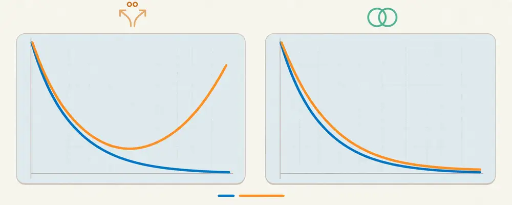
What a healthy curve looks like: Training error starts low (tiny datasets are easy to memorize) and rises as more data makes memorization harder. Validation error starts high and falls as the model sees more of the world. The two curves converge toward a shared level. The gap between them shrinks with data.

What an overfit curve looks like: A large, persistent gap between training error (low) and validation error (high) even as data grows. The model memorizes every training size you give it. This pattern says: the model has far more capacity than this data can support — simplify it, regularize it, or get much more data.

What an underfit curve looks like: Both curves converge, but to a high error level. More data will not help — the curves have already flattened at a bad value. The model is too simple or the features are wrong. This pattern says: add capacity or better features (Chapter 10).

The diagnostic power is that the same plot tells you which of the three regimes you are in. Students who skip learning curves often "fix" overfitting by collecting more data when the problem was model complexity, or "fix" underfitting with bigger models when the problem was bad features. The curve tells you which lever to pull.

Validation curves: error versus a hyperparameter

A validation curve fixes the data and varies one hyperparameter — tree depth, regularization strength, number of neighbors — plotting training and validation error against it.

The classic shape is a U for validation error: at low complexity (shallow tree, strong regularization), both errors are high — underfitting. As complexity rises, validation error falls. Past the sweet spot, training error keeps falling but validation error rises — overfitting. The bottom of the U is your hyperparameter choice, made by measurement, not gut feeling.

Validation curves also reveal the width of the good region. If the U is broad and flat, your choice is robust and you can say so in the paper. If it is a sharp narrow valley, your result is fragile — a reviewer who nudges the hyperparameter will get a different number, and you should report that honestly or choose a more stable model.

Worked example: diagnosing the rent model

You plot learning curves for the degree-15 polynomial from Chapter 1:

• At 50 training samples: train error Rs 200, validation error Rs 24,000. Huge gap.
• At 200 samples: train Rs 900, validation Rs 19,000. Gap barely moved.
• At 800 samples (you collected more): train Rs 3,400, validation Rs 11,000. Gap shrinking but still large.

Diagnosis: classic overfitting — persistent large gap, both errors still falling slowly with data. The curve also tells you data alone will not close this gap quickly; you would need perhaps 10,000 listings. The cheaper fix is to reduce complexity (Chapter 5) or regularize (Chapter 6).

Then you plot a validation curve over polynomial degree (1 to 15), with validation error:

• Degree 1: Rs 9,800 (underfit). Degree 3: Rs 6,100. Degree 5: Rs 6,400. Degree 8: Rs 9,200. Degree 15: Rs 19,000.

The U bottoms at degree 3–5. You choose degree 4 as a round, defensible value in the flat region, and you now have a figure for your paper that shows your hyperparameter choice was principled.

Reading curves during neural network training

For deep learning, the x-axis is epochs (training passes), not data size. Watch two curves per epoch: training loss (should fall steadily) and validation loss (falls, then flattens, then rises). The moment validation loss starts rising while training loss keeps falling is the exact moment memorization overtakes learning. That divergence point is where early stopping (Chapter 7) halts training — but you can only use it if you plotted the curves.

Practical details that matter: - Smooth the curves. Validation loss is noisy batch to batch; use a moving average or evaluate on the full validation set each epoch so the turning point is visible. - Log both loss and your real metric. Sometimes loss diverges while accuracy stays flat — know which one your paper reports and watch that one. - Save the plots. Every experiment's curves go into your lab records. When a reviewer asks why you chose epoch 42, you show the curve.

Learning curves beyond loss: accuracy, F1, and AUC

So far we plotted error (usually loss), but the same technique works with any metric — and you should plot the metric your paper actually reports. Two practical notes:

• Accuracy curves look different from loss curves. Loss can diverge (overfitting) while accuracy stays flat, because accuracy only cares about which side of the decision boundary a point falls on. If your paper reports accuracy, diagnose with accuracy curves; if it reports F1 or AUC, use those. The turning points can differ, and you want the curve that matches your claims.
• Use 5–8 data-size points, spaced multiplicatively. Train on e.g. 100, 200, 400, 800, 1600, 3200 samples — not 100, 200, 300, 400. Multiplicative spacing shows the trend with fewer expensive training runs, and the interesting behavior (the gap closing) usually happens across orders of magnitude.

One more diagnostic trick: plot the gap itself (validation error minus training error) against data size on a log scale. A gap that shrinks linearly on the log scale is healthy — it predicts roughly how much data you would need to close it fully. A gap that refuses to budge across a 10× increase in data is screaming that data is not your problem — go simplify or regularize.

When curves mislead

Learning curves assume your data-size subsamples are representative. If you subsample naively from imbalanced data, small subsets may contain zero minority-class examples, and the curve will show chaos that is really a sampling artifact — stratify every subset. Also, curves cost compute: for deep networks, training 6 models at increasing data sizes is expensive. A cheaper deep-learning habit is the single-run variant: train once on all data and watch per-epoch train/validation curves (Chapter 7's early-stopping plot). It answers a slightly different question — "am I overfitting during training?" rather than "would more data help?" — but it is nearly free.

Smoothing noisy curves

Real validation curves are jagged — one unlucky batch can spike the loss and fake a turning point. Three smoothing habits: evaluate on the full validation set (not a batch) at each checkpoint; apply a moving average over a small window before judging the trend; and require the trend to persist for several checkpoints before acting on it (the same "patience" idea as early stopping). When you publish the figure, plot both the raw faint line and the smoothed bold line — it shows honesty about the noise while keeping the trend readable. Reviewers trust a slightly noisy real curve more than a suspiciously perfect one.

For your research: Put a learning curve or validation curve figure in every empirical paper. It is one of the cheapest ways to signal competence to reviewers: it shows you measured the bias–variance tradeoff instead of guessing. When your curve shows overfitting, say so in the text and describe the defense you applied — reviewers trust authors who report the gap and address it far more than authors who report only a single triumphant accuracy number.

Key takeaways - Split data into train/validation/test; decide with validation, report with test. - Learning curves (error vs. data size) diagnose overfit, underfit, or healthy convergence. - Validation curves (error vs. hyperparameter) locate the complexity sweet spot by measurement. - A persistent train–validation gap means overfitting; converged-but-high errors mean underfitting. - In deep learning, watch per-epoch curves — divergence marks where memorization begins.

---

Chapter 4: More Data and Data Augmentation

Why data is the strongest defense

Return to the bias–variance decomposition: more data reduces variance. Intuitively, noise is random — with few samples, random quirks look like patterns (the gambler's red shirt). With many samples, quirks cancel out and only the true pattern survives. A model cannot memorize 100,000 varied examples the way it memorizes 300; memorization becomes more expensive than learning.

This is why the largest, most reliable gains in applied machine learning historically came from bigger datasets, not cleverer algorithms. Before reaching for exotic defenses, ask: can I get more data? Often the honest answer in a thesis is "some" — and Chapter 12's workflow shows how to make that "some" count.

What "more data" really means

Not all data additions are equal:

• More of the same (same hospital, same camera, same season) reduces variance but does not fix a dataset that misrepresents the real world. It helps with noise, not with bias in your sampling.
• More diverse data (new hospitals, new devices, new regions) is far more valuable. It attacks both variance and the hidden sampling bias that makes models fail in deployment.
• More of the hard cases (rare classes, edge conditions) improves the errors that actually matter. If your model fails on dark images, a thousand more bright images will not help.

When you write about your dataset, describe its diversity, not just its size. "5,000 images from three hospitals and two scanner models" is a stronger claim than "10,000 images from one clinic" — and reviewers know it.

Worked example: the crop-disease classifier

You are classifying wheat leaf images as healthy or diseased. You start with 800 images from one farm, one phone camera.

• Experiment 1 (800 images): train 98%, validation 74%. Overfit.
• You collect 3,000 more images from four farms, three phone models, morning and evening light. Train 91%, validation 86%.
• The gap shrank from 24 points to 5. You changed nothing about the model — the data did the work.

Notice the training accuracy fell. That is expected and good: the model can no longer memorize, so it must generalize. Students sometimes panic when train accuracy drops after adding data. It is a sign of health.

Data augmentation: manufacturing diversity

When collecting more real data is slow or expensive, data augmentation creates new training examples by transforming existing ones in ways that preserve the label. The key rule: the transformation must not change the correct answer.

For images: - Rotations, flips, crops, zooms (a diseased leaf is still diseased upside down) - Brightness, contrast, and color jitter (simulates different cameras and lighting) - Adding noise or slight blur (simulates sensor variation)

For text: - Synonym replacement, back-translation (translate to another language and back), paraphrasing - Random deletion or swapping of non-key words

For tabular data: - Adding small Gaussian noise to numeric features - SMOTE and its variants for oversampling minority classes (synthesize new minority samples between existing ones)

For audio: - Speed and pitch perturbation, background-noise mixing, time masking

What augmentation is really doing: it teaches the model invariance — "the label does not depend on rotation, lighting, or exact wording." Each augmented copy says: the pattern must survive this transformation. That is a powerful anti-memorization constraint, because memorizing pixel-exact images fails as soon as the pixels are rotated.

Augmentation done wrong

Three common mistakes:

1. Label-breaking transforms. Flipping a "6" versus "9" in digit recognition, or cropping out the tumor in medical images. If the transform can destroy the evidence for the label, it poisons training. Always verify transforms visually on samples from your own data.
2. Augmenting the validation/test set. Augmentation is a training-time defense. Your validation and test sets must reflect real, unaugmented data — otherwise you are measuring performance on a fantasy distribution.
3. Augmenting instead of fixing a broken dataset. If your data has systematic label errors or represents the wrong population, augmentation multiplies the problem. Fix collection first.

How much augmentation is enough?

There is no universal number, but there are measurement habits:

• Train with and without augmentation and compare validation curves. If the train–validation gap shrinks and validation improves, keep it.
• Start with mild, obviously-safe transforms; add aggressive ones only if mild ones underperform.
• In deep learning, augmentation is typically applied on the fly (each epoch sees differently transformed copies), which effectively multiplies your dataset by the number of epochs.

The research angle: augmentation as a contribution

Designing augmentation for a new domain is itself publishable work. "No standard augmentation exists for multispectral crop imagery; we propose domain-specific transforms based on agronomic knowledge" is a legitimate contribution — it encodes domain knowledge into the training process. Several published papers are exactly this: careful, validated augmentation schemes for medical, agricultural, or low-resource-language data. If your dataset is small and unusual, this may be your paper's core idea.

Synthetic data: manufacturing examples from scratch

Augmentation transforms real examples; synthetic data creates examples from nothing — simulations, generative models, or rule-based generators. It shines exactly where real data is scarcest:

• Rare classes. A fraud detector may have 2 million normal transactions and 300 frauds. A simulator encoding known fraud patterns can generate thousands of plausible fraud examples. (Pair with SMOTE-style interpolation between real minority samples for realism.)
• Physics you understand. If you can simulate it, you can train on it: electromagnetic simulations for antenna design, crop-growth models for yield prediction, rendering engines for object detection. The simulator encodes domain knowledge no dataset could match.
• Privacy-blocked domains. Medical and financial data often cannot be shared; synthetic datasets with matching statistics let collaborators develop methods without touching real records.

The validation rule for synthetic data is strict: never let synthetic data into your validation or test sets, and always report the real-data-only performance alongside any mixed result. A model that scores 95% on synthetic test examples and 80% on real ones is an 80% model — the simulator's simplifications are just another form of noise the model memorized. The honest paper says: "trained on 10,000 synthetic + 2,000 real images; all reported metrics on held-out real images." Reviewers accept synthetic training data readily when the evaluation is real; they reject it when the evaluation is synthetic too.

Pretraining: borrowing someone else's data

A cousin of synthetic data deserves mention: pretraining. Instead of manufacturing data, you start from a model trained on a massive public dataset (ImageNet for vision, large text corpora for language) and fine-tune it on your small dataset. The pretrained weights already encode general patterns — edges, textures, grammar — so your small dataset only needs to teach the task-specific part. This dramatically reduces overfitting on small data because the model is not learning everything from your 800 images; it is adjusting an already-sensible starting point. For student projects with limited data, fine-tuning a pretrained model with light regularization beats training from scratch in the large majority of cases — and "we fine-tuned a pretrained backbone" is a completely standard, reviewer-accepted methods sentence.

Test-time augmentation: a free second opinion

Augmentation has a lesser-known sibling: test-time augmentation (TTA). At prediction time, create several augmented versions of each test input (flips, crops, slight rotations), run the model on all of them, and average the predictions. The averaging smooths out the model's brittle reactions to any single view — a cheap ensemble with no extra training. Gains of 1–2 points are typical in vision tasks. Two cautions: it multiplies inference cost (fine for papers, sometimes too slow for deployment), and you must report whether your numbers use TTA — comparing your TTA score against someone else's single-view score is an unfair fight. State it plainly: "reported with 5-crop TTA" or "single center crop, no TTA."

Calibrating augmentation strength

A useful mental dial: augmentation strength should match your data scarcity. With 50,000 images, mild flips and crops suffice — the data already covers the variation. With 800 images, you need the heavy arsenal: strong color jitter, random erasing, mixup. The validation curve is your calibration tool here too: sweep augmentation intensity and watch the train–validation gap. If stronger augmentation keeps improving validation, you have not hit the limit; if validation degrades, you are distorting the data past recognition. There is no prize for the most aggressive pipeline — only for the one the curves endorse.

For your research: Document your augmentation pipeline as carefully as your model architecture: list every transform, its parameters, and the reasoning. Reviewers increasingly ask for this because augmentation choices can swing results by several percentage points — an undisclosed aggressive pipeline is a reproducibility hole. In your thesis, the learning-curve comparison (with vs. without augmentation) makes an excellent figure: it visually proves your defense worked.

Key takeaways - More data reduces variance; it is the strongest and most honest overfitting defense. - Diverse data beats merely larger data; hard cases matter most. - Data augmentation manufactures label-preserving variations to teach invariance. - Never augment validation/test sets; never use label-breaking transforms. - Falling training accuracy after adding data is a sign of health, not failure.

---

Chapter 5: Simpler Models, Fewer Features: Occam's Razor in Practice

The principle

Occam's razor — prefer the simplest explanation that fits the evidence — is not philosophy in machine learning. It is an empirical law: among models with similar validation performance, the simpler one almost always generalizes better, trains faster, is easier to debug, and is easier to publish honestly. Complexity must earn its keep with measured validation gains.

In practice this means a discipline: start simple, add complexity only when the curves (Chapter 3) justify it, and treat every added knob as guilty until proven innocent.

Choosing a simpler model family

The model family sets the ceiling on complexity. A sensible ladder for most student projects:

1. Linear/logistic regression — the honest baseline. If it works, stop. It is interpretable, fast, and nearly impossible to overfit badly.
2. Naive Bayes / k-NN — simple, with one or two hyperparameters.
3. Decision trees (shallow) — interpretable; depth is the complexity knob.
4. Random forests / gradient boosting — strong defaults for tabular data, but with more knobs.
5. Support vector machines — powerful with kernels, but kernel choice is a complexity decision.
6. Neural networks — the top of the ladder; reach for them when the data is large and unstructured (images, text, audio), not by default.

The research sin is starting at step 6 for a 500-row spreadsheet. Reviewers notice. A paper that reports "logistic regression: 84%, our 12-layer network: 85%" has actually published an argument for logistic regression. Always include the simple baselines — they are the control group of your experiment.

Constraining the complexity knobs

Every model family has knobs that control flexibility. Learn yours:

• Trees: maximum depth, minimum samples per leaf. A depth-3 tree is a simple model; a depth-30 tree is a memorization machine.
• k-NN: k itself. k=1 memorizes; larger k smooths.
• SVM: the C parameter (tolerance for misclassification) and kernel width. Small C and wide kernels are simpler.
• Neural networks: number of layers, layer widths. Width and depth are the capacity knobs.
• Polynomial regression: the degree.

The validation curve (Chapter 3) is how you set these knobs honestly: sweep the knob, plot validation error, pick the bottom of the U — or better, the simplest point within noise of the bottom.

Fewer features: the other half of simplicity

Every feature is an opportunity for the model to find a "red shirt" — a chance correlation. Irrelevant features do not just waste computation; they actively cause overfitting by giving variance more room to grow. Feature selection is an overfitting defense.

Three families of feature selection:

1. Filter methods — score each feature independently of the model: correlation with the target, mutual information, chi-squared tests. Fast, model-agnostic, and a good first pass. Remove features with near-zero variance or near-zero relationship to the target.
2. Wrapper methods — search subsets using the model itself: forward selection (add the best feature one at a time), backward elimination (remove the worst one at a time), recursive feature elimination. More accurate, much slower, and — warning — they can overfit the validation set if you search too aggressively.
3. Embedded methods — selection happens during training: L1 regularization (Chapter 6) drives useless weights to exactly zero. This is the modern default.

Domain knowledge beats algorithms. Before running any selection algorithm, ask a domain expert (or your literature review) which features should matter. A feature with a causal story is worth ten features with a correlation. In your paper, the feature list with justifications is part of the contribution.

Worked example: the rent model, simplified

Recall the Karachi rent prediction with the degree-15 polynomial disaster (train Rs 900, test Rs 19,000). Apply Occam's razor in two steps:

Step 1 — simpler model family. Replace the degree-15 polynomial with plain linear regression on the four original features. Result: train Rs 8,600, test Rs 9,000. The gap nearly vanishes. You have traded a spectacular training number for an honest one.

Step 2 — feature audit. You test each feature's contribution by removing it and watching validation error. Floor number barely matters (removing it changes validation error by Rs 60 — noise). Distance to main road matters enormously. You also discover "listing ID number" had accidentally been included as a feature — the polynomial was partly memorizing IDs, a classic leakage-adjacent mistake. Removing it and the useless feature, then refitting linear regression: train Rs 8,700, test Rs 8,800.

Two lessons: the final model is simpler and better, and the feature audit caught a data bug that no amount of regularization would have fixed cleanly.

The "simple baseline" publication strategy

For students, this chapter contains a whole publication strategy: beat the simple baseline honestly, or publish the simple baseline. Many applied papers are exactly this: "We show that on this new dataset, a regularized linear model matches published deep results at 1% of the cost." That is a real contribution — it corrects the literature's complexity bias. Reviewers respect it because it demonstrates the bias–variance understanding from Chapter 2: you identified that the problem's variance budget did not support the complex model.

When simplicity is wrong

Occam's razor is a tiebreaker, not a religion. If validation curves clearly show that added complexity keeps improving validation performance (not just training), take the complexity — the data is telling you the pattern is genuinely intricate. The razor says: do not pay for complexity you cannot measure.

Information criteria: AIC and BIC

Validation curves choose complexity by measurement, but there is an older, elegant alternative worth knowing: information criteria, which score a model as fit minus a complexity penalty, computed on the training data alone:

• AIC (Akaike): score = −2 × log-likelihood + 2 × (number of parameters). Lower is better.
• BIC (Bayesian): score = −2 × log-likelihood + log(n) × (number of parameters), where n is the sample size. Lower is better; the penalty grows with data, so BIC prefers simpler models than AIC on large datasets.

The idea is the bias–variance tradeoff in one formula: the likelihood term rewards fit (low bias), the parameter term punishes complexity (high variance). You fit several candidate models, compute AIC/BIC for each, and pick the lowest — no validation split needed, which is handy when data is too scarce to spare one.

Limitations you must know: AIC/BIC only work cleanly for models with a well-defined parameter count and likelihood — linear models, GLMs, ARIMA, mixture models. They break down for deep networks (what counts as a "parameter" when dropout is on?) and for models chosen by the data (the criteria assume the candidate set was fixed in advance). In modern ML practice, cross-validation has largely replaced them — but in statistics-flavored venues and for classical models, reporting "selected by BIC" is still respected. Know both languages: use CV for your neural nets, and reach for BIC when a reviewer from a statistics background asks how you chose your regression's complexity.

The one-standard-error rule

When a validation curve's bottom is flat, several complexity values are statistically tied. The one-standard-error rule says: pick the simplest model whose validation score is within one standard error of the best score. If depth-6 trees score 86.1% ± 1.2% and depth-12 trees score 86.8% ± 1.3%, the rule picks depth 6 — the extra complexity buys nothing you can distinguish from noise. This rule is Occam's razor made quantitative, and citing it in your paper ("complexity selected by the one-standard-error rule") signals unusual methodological maturity. It protects you from the most common self-deception in model selection: chasing a 0.7-point "win" that is really sampling noise.

Simplicity in the objective, not just the model

Occam's razor applies to your training objective too. A custom loss with four weighted terms and a hand-tuned schedule is a complexity liability: each term is a hyperparameter the reviewer cannot verify and a knob that can overfit the validation set. Prefer standard losses (cross-entropy, MSE) unless you can show, by ablation, that the custom term earns its keep on held-out data. The same goes for elaborate training schedules — if a plain constant learning rate with early stopping matches your fancy schedule within noise, publish the plain version. Simplicity compounds: a simple model with a simple loss and a simple schedule is a paper a reader can actually reproduce.

For your research: Structure your results table as a complexity ladder: baseline → +features → +model complexity → +defenses, with validation metrics at each rung. This table tells the reviewer a story: each step earned its place. If a complex step adds nothing, say so and keep the simpler model — that honesty is a signal of maturity that reviewers reward. And always ask of every feature: "What would I tell a reviewer this feature means?" If you have no answer, the feature is a liability.

Key takeaways - Among models with similar validation performance, choose the simpler one. - Start with simple baselines (linear/logistic regression) and climb the complexity ladder only with measured justification. - Every model family has complexity knobs — set them with validation curves. - Irrelevant features cause overfitting; select features with filters, wrappers, or embedded methods — plus domain knowledge. - Audit your feature list for leakage-adjacent bugs like IDs and timestamps.

---

Chapter 6: Regularization: L1 and L2, with Math Made Gentle

The core idea in one paragraph

Regularization says to the optimizer: fit the data, but keep the weights small. Instead of minimizing just the training loss, minimize training loss + penalty for large weights. The penalty is controlled by a strength parameter (usually called λ, lambda). Small λ: the model fits freely. Large λ: the model is forced toward simplicity. Tuning λ with a validation curve finds the sweet spot — this is the bias–variance tradeoff made into a single knob.

Why do small weights mean simpler models? A weight is the model's reliance on a feature. Huge weights mean the model's output swings wildly with small input changes — the definition of high variance, the wiggly overfit curve. Small weights mean smooth, stable, conservative predictions. Regularization is a leash on the model's excitability.

The two penalties

For a linear model with weights w₁, w₂, …, wₙ:

• L2 (Ridge): penalty = λ × (w₁² + w₂² + … + wₙ²). The sum of squared weights.
• L1 (Lasso): penalty = λ × (|w₁| + |w₂| + … + |wₙ|). The sum of absolute weights.

Same idea, one different exponent — but the behaviors differ in a way that matters enormously.

L2: the gentle shrinker

Squaring punishes large weights harshly and small weights lightly. A weight of 10 contributes 100 to the penalty; a weight of 0.1 contributes 0.01 — essentially free. So L2 shrinks all weights smoothly toward zero but rarely all the way there. Correlated features share the weight democratically: if two features carry the same signal, L2 splits the weight between them.

Use L2 as your default. It is stable, has a clean mathematical solution, and plays well with every optimizer including deep learning (where it is often called "weight decay").

L1: the strict selector

Absolute value punishes all weights equally per unit: reducing a weight from 10 to 9 saves exactly as much penalty as reducing 0.1 to 0. So the optimizer's best move is to push small, useless weights all the way to exactly zero and spend its penalty budget on the few weights that matter. The result: automatic feature selection. Out of 1,000 features, L1 might keep 40 and zero out the rest.

Use L1 when you suspect most features are irrelevant — genomics, text with huge vocabularies, sensor arrays. The surviving features are interpretable: "the model kept exactly these 40 genes" is a finding you can publish.

The geometry intuition (no equations needed)

Picture the penalty as a region the weights must stay inside — a budget. L2's budget is a circle (in two dimensions): smooth, no corners, so the best point usually touches the circle somewhere with both weights nonzero. L1's budget is a diamond: it has sharp corners on the axes, and the best point loves to land exactly on a corner — where one weight is zero. Corners create sparsity. That is the whole geometric story: circles shrink, diamonds select.

Worked example: regularizing the rent model

You fit linear regression on 20 features (the 4 real ones plus 16 derived interactions and ratios, several useless). Unregularized: train Rs 7,900, validation Rs 12,400 — the junk features are being exploited.

L2 sweep (λ from 0.001 to 100): - λ = 0.001: barely changes anything. Validation Rs 12,300. - λ = 1: weights shrink smoothly. Validation Rs 9,100 — the junk features are muted. - λ = 100: even useful weights are crushed. Validation Rs 11,500 — underfitting now.

Validation curve bottoms near λ = 1. Final: train Rs 8,900, validation Rs 9,050. The gap is nearly closed.

L1 sweep on the same data: - At the best λ, 13 of the 16 junk features get weights of exactly 0.000. The model kept area, rooms, distance to road, and two genuinely useful ratios. - Validation Rs 8,950 — same performance as L2, but now the model tells you which features matter.

You report both, choose L1 for the paper because the feature-selection story strengthens the contribution, and you include the validation-curve figure showing the λ sweep.

Elastic net: the best of both

When features are correlated (common in real data), pure L1 arbitrarily keeps one and kills its twins — unstable across data samples. The elastic net combines both penalties: λ₁×L1 + λ₂×L2. It selects groups of correlated features together while still zeroing the junk. If your paper uses high-dimensional correlated data, elastic net is the reviewer-approved choice — cite it as such.

Regularization in deep learning

In neural networks, L2 is usually called weight decay: each update shrinks weights slightly toward zero. It is nearly always on by default in modern training setups, and turning it off is a common beginner error behind "my network overfits instantly." Practical notes:

• Tune weight decay on a logarithmic scale (1e-5, 1e-4, 1e-3, …) — its effect is multiplicative.
• Do not regularize biases or normalization parameters; regularize only the weights. (Most frameworks handle this if you use their standard weight-decay option rather than adding the penalty manually.)
• L1 is rare in deep learning because exact zeros matter less when features are learned, not given.

Choosing λ without fooling yourself

The λ sweep must use the validation set, never the test set. A proper report: "λ was selected by 5-fold cross-validation over {0.001, 0.01, 0.1, 1, 10}; λ=1 minimized mean validation error." That one sentence, with the curve figure, preempts the reviewer's hardest question about your regularization.

The regularization path: watching weights die

One of the most informative plots in applied ML is the regularization path: fit the model at many λ values and plot each weight's value against λ (usually on a log scale). Reading it teaches you about your data:

• Weights that survive to large λ are your most robust predictors — the signal.
• Weights that collapse early were marginal — kept only when the penalty was weak.
• With L1, you literally watch weights die (hit exactly zero) one by one as λ grows, in order of increasing usefulness. The order of death is a feature-importance ranking, and it often disagrees with naive correlation rankings — because it accounts for redundancy between features.

Include this plot when L1 feature selection is part of your contribution. It shows reviewers how the selection behaved, not just the final survivor list.

Decision guide: which penalty when?

Situation	Choice	Why
Default, no strong reason otherwise	L2	Stable, smooth, works everywhere including deep learning
Many features, suspect most are junk	L1	Automatic sparse selection + interpretable survivors
Correlated features (sensors, genes, text)	Elastic net	Selects groups together; L1 alone picks arbitrarily among twins
Deep neural network	L2 as weight decay	Standard, well-supported by all frameworks
p >> n (more features than samples)	L1 or elastic net	L2 alone cannot zero out the noise dimensions
Need a stable feature list across resamples	Elastic net or L2	Pure L1's chosen set can flicker between data samples

One caution on that last row: if your paper's finding is "these 12 features matter," verify stability — run L1 on 10 bootstrap resamples and report how often each feature survives. A feature selected in 10/10 resamples is a finding; one selected in 3/10 is a rumor. Reviewers in bioinformatics and social science increasingly ask for exactly this stability check.

Standardize before you regularize

One mechanical step students routinely skip: standardize your features (zero mean, unit variance) before applying L1/L2. The penalty treats all weights equally, so a feature measured in thousands (area in sq ft) gets penalized far less per unit of influence than a feature measured in decimals — regularization ends up punishing the small-scale features hardest, which is arbitrary. Standardization puts every weight on the same scale so the penalty is fair. (Tree-based models do not need this, but regularized linear models and neural networks do.) If your λ sweep behaves erratically, unstandardized features are the first suspect.

For your research: Regularization is the single most expected defense in a methods section — its absence needs justification, not its presence. When you write it up, report three things: the penalty type (L1/L2/elastic net/weight decay), the λ selection procedure (grid + cross-validation), and the effect (e.g., "validation gap fell from Rs 4,500 to Rs 150"). If L1 selected features, list the survivors — that list may become a finding in your discussion. And remember the geometry: if a reviewer asks why you chose L1 over L2, "sparsity for interpretability" is a complete, respectable answer.

Key takeaways - Regularization minimizes loss + λ × penalty on weight sizes, trading fit for simplicity. - L2 (Ridge) shrinks all weights smoothly — the safe default, called weight decay in deep learning. - L1 (Lasso) drives useless weights to exactly zero — automatic, interpretable feature selection. - Elastic net combines both for correlated features. - Tune λ with validation curves or cross-validation on the validation set — never the test set.

---

Chapter 7: Dropout, Early Stopping, and Other Training-Time Defenses

Defenses that live inside training

Chapters 4–6 changed the data, the model, or the loss function. This chapter's defenses live inside the training loop itself: they change how the model learns, moment to moment. They are cheap, composable, and standard in deep learning — reviewers expect to see at least one of them whenever a neural network is trained on limited data.

Early stopping: quit while you are ahead

Recall the per-epoch curves from Chapter 3: training loss falls steadily; validation loss falls, flattens, then rises. Early stopping halts training at the bottom of the validation-loss valley instead of a fixed epoch count.

How to implement it properly:

1. Split off a validation set (or use a cross-validation fold).
2. After each epoch, evaluate validation loss on the full validation set.
3. Track the best validation loss seen so far; save the model weights at that point ("checkpointing the best").
4. If validation loss has not improved for patience epochs (e.g., 10–20), stop training.
5. Restore the best checkpoint — not the final weights.

Two subtleties students get wrong. First, patience: validation loss is noisy, so stopping at the first uptick quits too early; a patience of 10–20 epochs distinguishes noise from a real trend. Second, restore the best: the model at stopping time is already past the optimum — always roll back to the saved best weights, otherwise you kept the overfit version.

Why does it work? Early in training, the network learns broad, simple patterns (low effective complexity). Later it starts fitting noise (high effective complexity). Stopping early caps the effective complexity — it is regularization in the time dimension. There is even theory showing early stopping approximates L2 regularization.

Dropout: training an ensemble in disguise

Dropout randomly deactivates a fraction of neurons (typically 20–50%) during each training batch. Each batch therefore trains a slightly different sub-network. At test time, all neurons are active (with outputs scaled appropriately).

Why does this fight overfitting? Two views:

• The co-adaptation view: without dropout, neurons can become lazy — one neuron learns a feature and its neighbors learn to depend on it, building fragile chains. Dropout forces every neuron to be useful on its own, because its partners might vanish at any moment. The network learns redundant, robust representations.
• The ensemble view: training with dropout is approximately training an enormous ensemble of sub-networks that share weights, then averaging them at test time. Ensembles reduce variance — the same reason random forests beat single trees.

Practical rules:

• Apply dropout to fully connected layers; use it cautiously in convolutional layers (spatial structure makes naive dropout less effective — specialized variants exist).
• Typical rates: 0.2–0.5 for hidden layers. Higher rates on small datasets.
• Never apply dropout at test time (during final evaluation). Forgetting to disable it is a classic bug that silently degrades reported results.
• Dropout interacts with batch normalization — if you use both, check the literature for your architecture, because the combination can misbehave in some setups.

More training-time defenses

Batch normalization was invented to stabilize training, but it has a mild regularizing side effect: each batch's statistics are slightly noisy, which acts like injecting noise into the network — noise the model cannot memorize. It is not a replacement for dropout or weight decay, but it contributes.

Label smoothing replaces hard targets (1.0 for the correct class, 0.0 for others) with softened ones (e.g., 0.9 and 0.1 split among the rest). This stops the model from becoming overconfident — pushing weights to extreme values to output 0.9999 probabilities. Overconfidence is overfitting's close cousin: both come from taking the training data too literally.

Noise injection generalizes the idea: add small Gaussian noise to inputs, weights, or gradients during training. The model must learn patterns robust to perturbation — memorized noise does not survive. Data augmentation (Chapter 4) is the input-noise member of this family.

Stochastic depth / layer dropout (for very deep networks): randomly skip entire layers during training. Same philosophy as dropout, scaled up.

Gradient clipping is not an overfitting defense per se, but it belongs in the training loop: it prevents single batches from yanking weights violently, which keeps variance in check during unstable training.

Worked example: taming the wheat classifier network

Your wheat-disease CNN from Chapter 4 (3,800 images) still shows a gap: train 96%, validation 86%. You add training-time defenses one at a time, measuring each:

1. Baseline: train 96.2%, val 86.1%. Gap: 10.1 points.
2. + Early stopping (patience 15): training halts at epoch 38 instead of 100. Train 93.4%, val 87.3%. Gap: 6.1. (Cheaper and better.)
3. + Dropout 0.4 before the classifier head: train 91.8%, val 88.9%. Gap: 2.9.
4. + Label smoothing 0.1: train 91.2%, val 89.6%. Gap: 1.6. Calibration also improves — predicted probabilities now mean what they say.

Each defense shaved the gap while lowering training accuracy — the healthy signature from Chapter 4. The final model's validation number (89.6%) is the honest one, and the ablation table (each row = one defense added) is exactly the evidence reviewers want: it proves every component earned its place.

The interaction warning

Defenses compose, but not always additively. Heavy augmentation + high dropout + strong weight decay can push a model into underfitting — you will see it in the curves (Chapter 10): both train and validation errors stuck high. The professional move is the ablation study above: add defenses one at a time, watch the curves, and stop when the gap closes. More defense is not always better; enough defense is.

Mixup, CutMix, and stochastic weight averaging

Beyond the classics, three modern training-time defenses are worth knowing — all share the philosophy of "make memorization harder":

• Mixup trains on blends of examples: take two images, mix their pixels 70/30, and mix their labels 70/30. The model can no longer memorize exact training points because the training points themselves are moving targets; it must learn smooth transitions between classes. Two lines of code, surprisingly effective on small image datasets.
• CutMix pastes a rectangular patch from one image onto another, mixing labels proportionally to patch area. It forces the model to look at the whole image (a model fixating on one corner fails when that corner comes from another class) — a direct attack on spurious local correlations.
• Stochastic weight averaging (SWA) averages the weights from several late-training checkpoints instead of taking the final one. The average sits in a flatter, more stable region of the loss landscape — and flatter solutions generalize better (more on this in Chapter 9). It costs almost nothing: keep a running average of weights during the last stretch of training.

None of these replaces the fundamentals — data, regularization, honest validation. But when your ablation table needs one more row and the gap is nearly closed, these are respectable, well-cited options rather than exotic gambles.

Reproducibility note: seeds and nondeterminism

Training-time defenses involve randomness — dropout masks, augmentation draws, shuffled batches. That means two runs with different random seeds give slightly different results. For your paper: fix seeds for your main results, but also report the spread across 3–5 seeds ("89.6% ± 0.7%"). A defense whose benefit vanishes under a different seed is not a finding. And log the seeds — "seed 42" in your notebook is what makes your own work reproducible six months later.

Batch size as implicit regularization

A subtle training-time factor: batch size. Small batches produce noisy gradient estimates, and that noise acts like a regularizer — bouncing the optimizer out of sharp minima (Chapter 9) and preventing precise memorization. Very large batches give clean, exact gradients that settle into the nearest minimum, which is often sharp and overfit. This is one reason the "linear scaling rule" era of ever-larger batches came with generalization warnings. Practical guidance: if a model overfits and you are already using big batches for speed, try halving the batch size before adding heavier defenses — it is free regularization. Conversely, if training is unstable, larger batches calm it down. Treat batch size as a quiet member of your defense stack and report it.

For your research: Report your training-time defenses with the same precision as your architecture: "dropout 0.4 after each fully connected layer (disabled at inference), early stopping with patience 15 on validation loss, best checkpoint restored, label smoothing 0.1." Vague phrases like "we used dropout to prevent overfitting" are not reproducible — the rate, placement, and patience are the method. Include the ablation table; it is the most convincing paragraph of your results section because it shows causality, not just a final score.

Key takeaways - Early stopping halts at the validation-loss minimum; use patience and restore the best checkpoint. - Dropout trains an implicit ensemble of sub-networks, preventing fragile co-adaptation; disable it at test time. - Label smoothing, noise injection, and batch normalization add mild regularization through the training loop. - Add defenses one at a time (ablation) and watch the train–validation gap; too much defense causes underfitting. - Report exact rates, placement, and patience — vague "we used dropout" is not reproducible.

---

Chapter 8: Cross-Validation Done Right (and Common Mistakes)

Why a single split is not enough

A single train/validation split has a weakness: your conclusions depend on which samples landed in each split. With small datasets — typical in student research — one lucky split can make a mediocre model look brilliant, or one unlucky split can bury a good one. Cross-validation (CV) fixes this by rotating the split: every sample gets to be validation data exactly once, and you average the results.

K-fold cross-validation, step by step

1. Shuffle the dataset and divide it into K equal folds (K = 5 or 10 are standard).
2. For each fold i: train on the other K−1 folds, validate on fold i.
3. Record the validation metric for each fold.
4. Report the mean and standard deviation across folds.

The mean is your performance estimate; the standard deviation is its uncertainty. A result of "84% ± 6%" is honest. A result of "84%" from one split is a rumor. Always stratify for classification: each fold should contain the same class proportions as the full dataset, otherwise a fold missing a rare class produces a meaningless score.

What cross-validation is for — and what it is not for

CV estimates how well your modeling procedure generalizes. It is the right tool for:

• Comparing models or hyperparameters (pick the one with the best mean CV score).
• Reporting expected performance on small datasets where a single held-out test set would be too noisy.
• Tuning λ in regularization (Chapter 6) or the complexity knobs (Chapter 5).

CV is not a way to train your final model on more data — though in practice, after CV selects the procedure, you retrain on all the data for the deployed model. And CV does not replace a true held-out test set when you have enough data: with 100,000 samples, a single clean split is fine and far cheaper.

Nested cross-validation: tuning without lying

Here is the trap: if you use CV to choose the best hyperparameters and then report the best CV score as your result, that score is optimistic — you selected the winner using the validation folds. The honest procedure is nested CV:

• Outer loop: splits data into train/test folds to estimate performance.
• Inner loop: within each outer training set, runs its own CV to select hyperparameters.
• The outer test fold is never touched during tuning.

Nested CV costs K×K trainings, which is expensive — but it is the correct answer when a reviewer asks, "Was your reported number tuned on the data it was measured on?" For a thesis with a small dataset and big claims, nested CV is worth the compute.

Worked example: honest model selection on the rent data

You have 400 listings and three candidates: linear regression, degree-3 polynomial, degree-3 polynomial with L2 (λ=1). Procedure:

1. 5-fold CV for each candidate (no test set touched — you will do nested properly):
2. Linear: 9,050 ± 420
3. Poly-3: 6,300 ± 510
4. Poly-3 + L2: 6,050 ± 380
5. Poly-3 + L2 wins on mean and has the lowest variance across folds — a double signal.
6. Nested check: outer 5-fold CV, inner 3-fold CV for λ selection. Mean outer score: 6,120 ± 460. Slightly worse than the naive number — that difference is the optimism you just removed.
7. You report 6,120 ± 460 as the honest estimate, retrain Poly-3 + L2 on all 400 listings for deployment, and note the procedure in the paper.

A classmate does it wrong: tries 20 hyperparameter settings, picks the best single-split validation score, reports it as the result. Their number looks 8% better than yours. Their number is also fiction. Yours survives review; theirs does not.

The leakage catalog: six common mistakes

1. Tuning on the test set. The cardinal sin. Every peek — "let me try one more setting and check the test score" — biases the test number upward. Lock the test set away (literally: separate file, no loading until the end).

2. Preprocessing on the full dataset. Computing normalization statistics, imputing missing values, or selecting features using all the data before splitting leaks information across the split. The rule: fit every preprocessing step on the training fold only, then apply to validation. In code, this means pipelines — preprocessing inside the CV loop, not before it.

3. Feature selection before splitting. Selecting the "best" 50 of 5,000 features on the full dataset, then cross-validating, is one of the most published forms of leakage. The selection saw the validation labels. Do selection inside each fold.

4. Duplicate or near-duplicate samples across splits. In medical imaging, multiple scans from the same patient must stay in the same fold — otherwise the model "recognizes the patient" instead of the disease. Use group-aware splitting (GroupKFold) whenever samples cluster by patient, farm, device, or time period.

5. Time-series shuffling. For temporal data, random K-fold lets the model train on the future and validate on the past. Use time-ordered splits: train on earlier periods, validate on later ones. The future must never inform the past.

6. Augmentation before splitting. Augmenting the dataset and then splitting puts near-copies of the same image in both train and validation — the model memorizes the original and is "tested" on its rotation. Split first, augment only the training folds.

The one-sentence audit for your own work

Before submitting anything, ask: "Did any number, statistic, or decision that shaped the model come from data the model is evaluated on?" If yes — including through preprocessing, selection, or a casual peek — redo it cleanly. This single question catches all six mistakes.

LOOCV, repeated K-fold, and the compute budget

K-fold has two relatives worth knowing:

• Leave-one-out CV (LOOCV): K equals the dataset size — each sample gets its own fold. It is nearly unbiased (each training set is almost the full dataset) but has high variance as an estimator (the training sets overlap almost completely, so the fold scores are highly correlated) and costs N trainings. Use it only for tiny datasets (N < 100) with cheap models. For anything else, it is the worst of both worlds: expensive and noisy.
• Repeated K-fold: run 5-fold CV several times with different shuffles and average everything. This shrinks the variance that comes from any single lucky/unlucky partition. When your paper's headline comparison is a 1–2 point difference between methods, repeated CV (say 5 repeats of 5-fold = 25 trainings) is what makes the comparison credible. Report "repeated 5-fold CV (5 repeats), mean ± std."

Budgeting rule of thumb: spend compute in this order — (1) one honest K-fold to pick the approach, (2) repeated K-fold to confirm close comparisons, (3) nested CV only when you tuned extensively and need an unbiased final estimate. Do not spend your GPU budget on nested CV for a model you have not yet shown beats the baseline — diagnose cheaply, confirm expensively.

Shuffling, seeds, and the "lucky split" problem

Every CV involves shuffling, and shuffling involves a random seed. A dirty secret of the field: some published improvements are just lucky seeds. Protect yourself: fix a seed for reproducibility, but verify your conclusion holds across 2–3 different seeds before claiming victory. If method A beats method B on seed 1 but loses on seeds 2 and 3, you have no finding — you have noise. Stating "results held across three random seeds" in your paper is a small sentence that buys a lot of reviewer trust.

Reporting CV: what numbers to publish

A complete cross-validation report fits in one line per method: "5-fold stratified CV: 86.2% ± 1.4% (seeds 1–3)." Include the K, stratification/grouping, the number of repeats, and the seeds — everything needed to reproduce the spread, not just the mean. When comparing two methods, report the paired difference per fold ("our method beat the baseline by +2.1 ± 0.9 points across folds") rather than two independent means; paired comparison removes fold-to-fold variation and is the statistically honest way to claim an improvement. If the paired difference's error bar crosses zero, say so — "no significant difference" is a publishable finding that saves the field from a false lead.

For your research: Your methods section should contain a "validation strategy" paragraph that a reviewer can audit: the split ratios or K, stratification, what was tuned and on which data, and the explicit statement "the test set was used only for final reporting." Name your leakage controls: "normalization statistics were computed on training folds only; patient-level grouping was enforced in all splits." These two sentences preempt the most damaging reviewer objection — that your numbers are inflated — and they cost you nothing but discipline.

Key takeaways - K-fold CV rotates the validation split; report mean ± standard deviation, stratified for classification. - Use nested CV when hyperparameters are tuned — otherwise the reported score is optimistic. - Fit all preprocessing, feature selection, and augmentation inside the training folds only. - Watch for group leakage (same patient/farm in both splits) and time leakage (shuffling temporal data). - Audit with one question: did any decision that shaped the model come from evaluation data?

---

Chapter 9: Overfitting in Deep Learning (Memorization, Double Descent Concept)

The paradox that broke the old rules

Classical theory (Chapters 1–8) says: a model with more parameters than training samples should memorize and fail. A modern neural network routinely has millions of parameters and trains on thousands of images — by the old rules, a memorization catastrophe. Yet these networks generalize remarkably well. Understanding why — and where the old rules still bite — is essential, because deep learning is where most student researchers meet overfitting in its strangest form.

Memorization: networks can fit anything, including nonsense

The landmark demonstration is simple and shocking: take a standard image dataset, randomly shuffle all the labels (so the images mean nothing), and train a deep network. It still reaches ~100% training accuracy. The network has enough capacity to memorize every single training example individually, noise and all.

This proves two things. First, capacity is not understanding — fitting the training set tells you nothing about what was learned. Second, since the same network does generalize on correctly labeled data, something beyond mere capacity must explain generalization. The network is not forced to generalize by lack of room; it prefers simple patterns when they exist. Researchers call this implicit bias: gradient-based training tends to find simple, smooth solutions first (broad patterns early, memorization late — which is exactly why early stopping works).

The practical consequence: in deep learning, "my model fits the training data" is the weakest possible evidence. Everything must be validated on held-out data, always, with the disciplines of Chapters 3 and 8.

Why deep networks still overfit (the ordinary ways)

The paradox does not mean deep networks are immune. They overfit constantly, through familiar channels:

• Small datasets. A million-parameter network on 500 images will memorize — the implicit bias toward simplicity is overwhelmed when there is almost nothing simple to find. This is the most common student scenario.
• Label noise. Mislabeled examples get memorized late in training, degrading the decision boundary. Cleaning labels often beats adding defenses.
• Too-long training. The network learns patterns first and noise later; training past the validation minimum (Chapter 7) walks straight into memorization.
• Spurious correlations. The network learns the easiest predictive signal, not the right one: hospital A's scanner artifacts instead of disease signs, image backgrounds instead of objects. This is overfitting to dataset quirks at scale — and it survives train/test splits when the test set shares the same quirks.

That last point deserves emphasis: a test set drawn from the same biased source as the training set will not catch spurious correlation. If all your diseased wheat photos were taken on cloudy days, the network may learn "cloudy = diseased" and ace your test set — then fail on a sunny farm. The defense is out-of-distribution testing: evaluate on data from a new source (new hospital, new farm, new camera) and report that number alongside the in-distribution one.

Double descent: the curve that dips twice

The classical U-curve (Chapter 2) says test error falls, then rises with complexity. In deep learning, researchers found something stranger: past the point where the model becomes large enough to perfectly interpolate the training data (zero training error), test error can start falling again. The curve descends, ascends, then descends a second time — double descent.

An intuitive reading: in the first descent, the model is too small and behaves classically. Near the interpolation threshold, the model is just barely big enough to memorize — it contorts itself into strained, fragile fits (peak error). Far beyond the threshold, with vastly more parameters than needed, the optimizer has room to find a smooth interpolating solution — memorization without contortion, and smooth solutions generalize. Bigger becomes better again, provided you can afford it.

What should a student researcher do with this? Three grounded lessons:

1. Do not fear large models on principle — but do not assume they generalize either. Double descent describes a tendency, not a guarantee; your validation curves are still the law.
2. The interpolation regime is dangerous. Models just big enough to fit the training data are often the worst generalizers. If you must use a small network, regularize it; if you can use a much larger one with proper defenses, it may paradoxically do better.
3. Report model scale. "We used a 110M-parameter model" is relevant methods information now, because scale interacts with generalization in ways reviewers understand.

The modern deep-learning anti-overfitting stack

In practice, the community converged on a standard stack — use it as your default and ablate from there (Chapter 7):

• Data: as much as possible, plus aggressive augmentation (Chapter 4).
• Architecture: appropriate inductive bias — convolutions for images, attention for sequences. The right structure is itself an overfitting defense because it restricts what kinds of patterns can be learned.
• Training: weight decay (L2), dropout where suitable, label smoothing, early stopping with best-checkpoint restore.
• Evaluation: held-out test set plus out-of-distribution evaluation; learning curves saved for every run.

Note what is not on the list: exotic tricks. The standard stack, applied carefully, beats a exotic trick applied hopefully, and it is far easier to describe honestly in a paper.

Worked example: the sunny-farm failure

You train the wheat-disease CNN. In-distribution results look excellent: validation 91%, test 90.5% (same farms, same cameras). You deploy the demo to a new partner farm — accuracy collapses to 63%.

Diagnosis with the tools of this book: you collect 200 images from the new farm and test. Error analysis shows the model keys on soil color in the background — your training farms had dark soil when disease was present (a seasonal coincidence), and the network learned the easy signal. This is spurious correlation: a form of overfitting invisible to your test set because the test set shared the quirk.

Fixes, in order: (1) augment backgrounds aggressively (random crops that exclude soil, background replacement); (2) collect training images across soil types and seasons — diversity (Chapter 4); (3) add an out-of-distribution farm to your validation protocol permanently, and report both numbers in the paper. Final honest report: 90.5% in-distribution, 81% on the new farm, with the gap discussed rather than hidden. That discussion paragraph is what makes the paper trustworthy.

Sharp vs. flat minima: why some fits generalize

Picture the loss landscape as terrain. Training finds a valley (a minimum). Some valleys are sharp — narrow crevasses where a tiny step in any direction spikes the loss. Others are flat — wide basins where the loss stays low across a broad region. Research strongly suggests flat minima generalize better: a sharp minimum is a precise memorization of the training sample — shift the data slightly (as new data does) and you climb out of the crevasse. A flat minimum is robust — the same weights work across data variations.

This explains several phenomena at once: why small-batch training often generalizes better than large-batch (noisier updates bounce out of sharp crevices into flat basins), why weight averaging (SWA, Chapter 7) helps (averaging lands in flat regions), and partly why overparameterized networks generalize (huge parameter spaces contain vast flat regions the optimizer can settle into). As a mental model for your work: whenever a technique adds noise, averages, or smooths, ask "is this pushing me toward flatter minima?" — if yes, it is probably helping generalization.

Grokking: memorization that turns into understanding

One of the strangest recent observations: on some algorithmic tasks, a network first memorizes the training data (perfect train accuracy, terrible validation) — and then, after much longer training, validation accuracy suddenly jumps to perfect. The network "groks" the underlying rule long after it finished memorizing. Memorization was not the end state; it was a phase.

Grokking is mostly observed on synthetic tasks, and its practical relevance is still debated — but it carries a conceptual lesson worth keeping: the training/validation gap at one moment in training is not the whole story. Combined with double descent, it completes this chapter's warning: in deep learning, the relationship between fitting and generalizing is genuinely weirder than the classical U-curve. Your defenses against that weirdness remain the same — hold out data honestly, evaluate out-of-distribution, and let the curves, not the theory, have the last word.

For your research: If your paper uses deep learning, reviewers will probe exactly the failure modes of this chapter: "How do you know it isn't memorizing? What happens on data from a new source?" Answer before they ask: report training vs. validation vs. test and an out-of-distribution evaluation; describe your augmentation and regularization stack precisely; include the ablation table. A paper that discusses its generalization limits is stronger than a paper that pretends they do not exist — the former gets cited, the latter gets a skeptical review.

Key takeaways - Deep networks can memorize even random labels — fitting training data proves nothing about understanding. - Gradient training prefers simple patterns first (implicit bias), which is why early stopping works. - Spurious correlations survive in-distribution test sets; evaluate out-of-distribution. - Double descent: past the interpolation point, much larger models can generalize better — but validate, don't assume. - The standard stack (data + augmentation + weight decay + dropout + early stopping + OOD evaluation) is your default.

---

Chapter 10: Underfitting: The Other Side of the Coin

The student who never opened the book

Chapter 1's memorizing student overfits. His classmate underfits: she skimmed the syllabus once, learned almost nothing, and scores 45 on every exam — last year's paper and the new one alike. Underfitting is failure to capture even the training pattern: high bias, low training performance, and no gap to diagnose because there is nothing to generalize.

Underfitting gets less attention than overfitting, but it wastes just as much researcher time — especially now, when heavy-handed defenses (Chapter 7's interaction warning) can push a model from overfit straight past the sweet spot into underfit.

Recognizing underfitting in the curves

From Chapter 3, the signature is unmistakable: training error and validation error converge — but to a high value. The gap is small (no overfitting), yet performance is poor (no learning). More data will not help: the curves have flattened at a bad level, which means capacity or features, not data, are the bottleneck.

Common causes, in rough order of frequency:

1. Model too simple — linear model on nonlinear data, tree too shallow, network too small.
2. Over-regularization — λ too large, dropout too high, early stopping with too little patience. The defenses became the disease.
3. Bad features — the information needed simply is not in the inputs. No model can learn what is not there.
4. Under-training — too few epochs, learning rate too low, optimization stuck. The model could fit but was not allowed to.
5. Label noise or wrong problem framing — if 20% of labels are wrong, or the task as defined is genuinely hard, even a good model plateaus. Check the noise floor (Chapter 2).

The underfitting fix ladder

Diagnose first, then climb:

1. Check the curves. Small gap + high error = underfitting confirmed. Large gap = overfitting — you are in the wrong chapter.
2. Loosen the defenses. Reduce λ, lower dropout, extend patience. Re-measure. Many "mysterious" underfits are just over-regularization.
3. Add capacity. Deeper tree, wider network, higher-degree features, weaker regularization. Move right along the validation curve toward the U's bottom.
4. Engineer features. Add interactions, domain-informed transformations, or better representations. Often cheaper than a bigger model.
5. Train longer and better. More epochs, tuned learning rate, better optimizer settings. Verify training loss is actually still decreasing — if it plateaued high, the optimizer may need help, not time.
6. Question the data. Audit labels on a sample; check class balance; verify the features contain the signal. Some underfits are data problems wearing a model costume.

Worked example: the over-defended classifier

A student builds a loan-default classifier on 5,000 tabular records. Worried about overfitting (she read Chapters 1–9 a little too eagerly), she applies everything: aggressive L2 (λ=10), dropout 0.5, early stopping with patience 3, heavy feature pruning.

Results: train 68%, validation 67%. The gap is tiny — no overfitting. But 68% is barely above the 62% majority-class baseline. The learning curves show both errors flat and high from epoch 5 onward.

Fix ladder applied: (1) curves confirm underfitting; (2) she relaxes λ to 0.1, dropout to 0.2, patience to 15 — validation rises to 74%; (3) she restores two pruned features with domain justification (employment length, existing debt ratio) — validation 78%; (4) trains to convergence — final train 81%, validation 79%. The gap is a healthy 2 points and the model is genuinely useful. The lesson: defenses are medicine — the dose matters, and overdose is a diagnosis too.

Underfitting in deep learning: the capacity check

A quick deep-learning diagnostic: can your network overfit a tiny subset? Train on just 50 samples with defenses off. If it cannot reach near-100% training accuracy on 50 samples, something is structurally wrong — broken architecture, bug in the loss, learning rate far too low, or data pipeline error. A healthy network should memorize a tiny subset effortlessly. Only once it passes this "can it overfit at all?" check do you re-enable defenses and scale up. This single test saves days of confused hyperparameter tuning.

The balanced view: navigating the whole curve

Keep the full picture from Chapter 2 in mind. Your job is not "avoid overfitting" — it is find the bottom of the U:

• Far left (underfit): both errors high, small gap → add capacity, loosen defenses, improve features.
• Bottom (good fit): validation minimized, small healthy gap → stop, report, publish.
• Far right (overfit): large gap → the defenses of Chapters 4–7.

Every experiment moves you along this curve. The curves tell you where you are; the fix ladder tells you which direction to step. Researchers who internalize this stop thrashing between random hyperparameter guesses and start navigating.

Knowing when to stop: the irreducible-error floor

Not every underfit is fixable — some tasks are just hard, and knowing when you have hit the floor saves months. Three ways to estimate the floor:

1. Human-level performance. Have a domain expert do the task on a sample of your test data. If experts agree with each other only 88% of the time, 88% is roughly your ceiling — a model at 86% is essentially done, and chasing 95% means fitting label noise. Report the human baseline in your paper; it reframes "only 86%" as "near human-level."
2. Inter-annotator agreement. If you have multiple labelers, their disagreement rate directly estimates label noise. A dataset with 12% annotator disagreement cannot honestly support claims above ~88% accuracy.
3. The plateau test. If learning curves flatten with more data, capacity increases, and better features all fail to move validation error, you are likely at the noise floor. Document the attempts — "increasing depth from 4 to 12 layers and doubling the data changed validation accuracy by less than 0.5%" — and declare the floor in your discussion. That is a result, not a failure: you have characterized the problem's difficulty.

The research mistake is the opposite: assuming every gap between your score and 100% is a model deficiency, then adding complexity until the model overfits the noise in pursuit of an unreachable number. The bias–variance decomposition from Chapter 2 is your license to stop: once bias and variance are both small relative to the irreducible noise, you are done. Write it up.

Underfitting as a deliberate choice

Finally, note that underfitting is sometimes strategic. In high-stakes settings — medical triage, loan approval — a slightly underfit, heavily regularized model with stable, conservative predictions is preferable to a sharper model with a 2-point higher validation score but wilder behavior on edge cases. "We chose the simpler configuration" is a defensible, even admirable, methods sentence when the deployment context demands reliability over leaderboard scores. The U-curve's bottom is not always the deployment optimum; sometimes a step left of the bottom is the responsible choice. Say so explicitly, and reviewers will respect the judgment.

Underfitting vs. concept drift: a diagnostic trap

One more trap: a model whose performance decays over time can look like underfitting in disguise. Suppose your classifier scored 85% at launch and now scores 72% on recent data, with retraining on recent data failing to recover. The learning curves on recent data show the classic underfit signature — high flat errors. But the cause is not capacity; it is concept drift: the world changed (new fraud patterns, new slang, new crop varieties), so the old features no longer carry the signal. More capacity cannot fix a stale feature set. The diagnostic: train on recent data only — if a fresh model on fresh data performs well, the old model suffered drift, not underfitting. The fix is data refresh and feature renewal, not a bigger network. In your paper's future-work section, naming drift as a limitation ("performance should be re-validated as language use evolves") shows you understand the model's shelf life.

The two-minute underfitting triage

When curves show the underfit signature, run this triage before the full fix ladder: (1) glance at training loss — still decreasing? Then just train longer; (2) check your regularization settings — did you leave last week's aggressive λ or dropout in place? Loosen and re-run; (3) ask whether the features could possibly contain the answer — if a human expert cannot predict the label from the features you provided, no model can. These three checks resolve the majority of underfits in minutes, because most underfits are under-training, over-defense, or missing information — in that order.

For your research: Underfitting is underreported in papers because it is embarrassing — nobody publishes "our model failed to learn." But your thesis or lab notebook should document the underfit attempts: they prove you explored the complexity space systematically rather than lucking into one working configuration. In the paper's discussion, one honest sentence — "Simpler configurations underfit (validation accuracy below 70%), indicating the task requires the reported capacity" — turns a dead end into evidence that your final model choice was principled.

Key takeaways - Underfitting = high bias: both train and validation errors high with a small gap; more data will not fix it. - Common causes: too-simple model, over-regularization, bad features, under-training, noisy labels. - Fix ladder: confirm with curves → loosen defenses → add capacity → engineer features → train better → audit data. - Deep-learning sanity check: a healthy network should memorize 50 samples with defenses off. - Your goal is the bottom of the U-curve, not merely "not overfit."

---

Chapter 11: Case Studies: Overfitting Failures and What Reviewers Look For

Why study failures

Every technique in this book exists because someone learned it the hard way — in a retracted claim, a failed deployment, or a brutal peer review. This chapter walks through five realistic failure cases, each mapped to the chapter that would have prevented it. Read them as cautionary tales and as a preview of your reviewer's mindset: reviewers are pattern-matching your paper against failures they have seen before.

Case 1: The 99% classifier that knew nothing

A student team built a pneumonia detector from chest X-rays, reporting 99% accuracy — better than published state of the art. At review, an expert noticed the test set came from the same two hospitals as the training set. A follow-up evaluation on scans from a third hospital scored 71%. Investigation revealed the model had learned each hospital's scanner watermark and text overlays: hospital A's machine (more pneumonia cases in the sample) stamped images differently than hospital B's. The model was a watermark detector.

Failure: spurious correlation (Chapter 9) plus in-distribution-only testing. Prevention: out-of-distribution evaluation, error analysis on what the model learned (saliency maps would have shown attention on the watermark, not the lungs). Reviewer lesson: "impressive accuracy on a dataset with known confounds" triggers the question what did it actually learn? — answer with evidence, not accuracy.

Case 2: The tuned-to-death benchmark

A researcher compared 40 model configurations on a public benchmark's test set, iterating for weeks, and reported the best score as "our method achieves 94.2%." The paper was rejected: the test set had been used as a validation set 40 times over. The reported number measured the luckiest of 40 draws, not the method. When the area chair re-ran the winning configuration on a fresh split, it scored 89%.

Failure: test-set peeking / leakage (Chapter 8). Prevention: lock the test set; tune on validation or nested CV; report the selection procedure honestly. Reviewer lesson: a suspiciously round-beating number with many ablated variants and no validation protocol described is a red flag. Describe your protocol before they ask.

Case 3: The feature-selection mirage

A genomics study selected 30 "predictive" genes from 20,000 candidates using the full dataset, then cross-validated a classifier on those 30 genes, reporting 92% accuracy. A reviewer re-ran the analysis with selection inside each fold: accuracy fell to 61% — barely above chance. The gene list was noise that happened to correlate in that sample; the CV after selection could not detect it because the selection had already seen all the labels.

Failure: feature selection before splitting (Chapter 8, mistake #3). Prevention: pipelines — selection inside the fold. Reviewer lesson: in high-dimensional data, reviewers check where selection happened. "We selected features then cross-validated" is an instant objection; "selection was performed independently within each training fold" is an instant pass.

Case 4: The deployment collapse

A crop-yield model trained on three seasons of data from one region achieved excellent cross-validated scores. Deployed the next season in a neighboring region, its predictions were useless. The model had fit region-specific planting-calendar quirks and that period's weather anomalies — patterns that did not transfer across space or time. The business lost a season of trust.

Failure: non-representative data treated as representative (Chapter 4); temporal/spatial leakage in validation — random folds mixed seasons, so validation never tested "a future season" (Chapter 8, mistake #5). Prevention: time-ordered and group-ordered validation; diverse data collection; honest discussion of the deployment distribution. Reviewer lesson: for applied papers, "will this work next year / next door?" is the real question. Validation that respects time and grouping answers it.

Case 5: The over-defended thesis

A master's student, terrified of overfitting after a harsh seminar, regularized her small text classifier into the ground: heavy dropout, tiny network, aggressive early stopping. Her results underperformed a plain logistic baseline. Her examiner's verdict: "You optimized for not-being-wrong instead of being right." She removed half the defenses, the model improved by 9 points, and the thesis passed — with a new section analyzing the bias–variance tradeoff of her defense choices.

Failure: underfitting via over-defense (Chapter 10). Prevention: the fix ladder; ablations showing each defense's contribution; remembering the goal is the bottom of the U, not the left edge. Reviewer lesson: reviewers can spot fear-driven underfitting too — a model weaker than its own baseline invites the question why is the sophisticated method worse?

The reviewer's checklist (use it on yourself first)

Experienced reviewers scan for overfitting with a mental checklist. Run your paper through it before submission:

1. Is there a clean test set, used once? Stated explicitly in the methods.
2. Are train, validation, and test numbers all reported? A missing training number hides the gap.
3. Was anything tuned on the test set? Including "we tried a few things and kept the best test score."
4. Did preprocessing/selection happen inside the folds? Pipelines, not pre-split computation.
5. Are the splits appropriate to the data? Grouped by patient/farm/device; time-ordered for temporal data.
6. Is there an out-of-distribution check? New source, new time period — at least discussed.
7. Do the defenses match the data size? A huge network on 400 samples with no regularization is a flag; so is a trivial model that "beats" deep baselines without explanation.
8. Are uncertainty and ablations reported? Mean ± std across folds/seeds; each component justified.
9. Does the claim respect the noise floor? Accuracy near 100% on noisy real-world labels invites disbelief.
10. Is the limitation section honest? "Performance may degrade on data from unseen hospitals" is a strength, not a weakness.

A paper that passes all ten is rare — and that rarity is exactly why it gets accepted.

Worked example: pre-submission audit

You are about to submit the wheat-disease paper. Audit:

• Train/val/test: 91.2 / 89.6 / 89.1 — gap small, all reported. ✓
• λ, dropout, patience tuned on validation; test set locked in a separate file until final week. ✓
• Normalization statistics from training folds only; augmentation on training folds only. ✓
• Images grouped by farm in splits (GroupKFold) — no farm in both train and validation. ✓
• Out-of-distribution: new farm scored 81%; reported and discussed. ✓
• 5-fold CV: 89.6 ± 1.8; ablation table for each defense. ✓
• Limitations paragraph written. ✓

You submit knowing the reviewer's checklist is already satisfied. Whatever they criticize, it will not be the experimental hygiene.

Case 6: The target-derived feature

A credit-risk team built a loan-default predictor with an impressive AUC of 0.97. During audit, someone asked what the top feature was: "days_since_last_missed_payment." The problem: for loans that never defaulted, this field was filled with a placeholder computed at the end of the observation window — a value that implicitly encoded "this loan survived." The feature was derived from the outcome it was predicting. Removing it dropped AUC to 0.78 — the honest number.

Failure: target leakage through feature engineering (Chapter 8's leakage family — the subtlest member, because the split was clean and the CV was correct; the poison was in the features themselves). Prevention: the "time-travel test" — for every feature, ask: "Would this value have been knowable at prediction time for a genuinely new case?" Any feature computed using information from after the prediction moment is leakage. Timestamp every feature's knowledge cutoff during data construction. Reviewer lesson: reviewers in applied ML now routinely ask for the feature list with definitions. A feature whose definition mentions the outcome or the future is an instant rejection. Write the time-travel justification for each non-obvious feature in your appendix or supplementary material.

The meta-lesson of all six cases

Notice the pattern: in every case, the researchers were competent, the code ran, and the numbers looked great. Overfitting failures are not stupidity failures — they are design failures, invisible from inside the experiment and obvious from outside it. That is why the defenses in this book are structural (locked test sets, pipelines inside folds, grouped splits, OOD evaluation) rather than advisory ("be careful"). Structure beats willpower. And the cheapest structural defense of all is a second pair of eyes: none of these six failures would have survived a colleague asking "show me the gap" before submission. Build the structure in Chapter 12's workflow, and these six cases become stories about other people.

For your research: Before every submission, perform this audit literally — print the ten-point checklist and tick it against your manuscript. Better: ask a colleague to audit your paper as a hostile reviewer whose job is to find the overfitting. Every flaw they find before submission is a rejection you avoided. And when you review others' papers, apply the same checklist generously but firmly: the community's quality depends on reviewers who check the gap, not just the headline number.

Key takeaways - The classic failures: spurious correlation, test-set tuning, pre-split feature selection, non-representative validation, over-defense. - Reviewers pattern-match your paper against these failures — preempt them with explicit methods text. - Report train/val/test, use pipelines inside folds, group and time-order splits appropriately, evaluate out-of-distribution. - An honest limitations section is a strength. - Audit your own paper with the ten-point checklist before submission.

---

Chapter 12: Checklist: An Overfitting-Proof Experimental Workflow

From knowledge to habit

You now know the theory (Chapters 1–2), the diagnostics (Chapter 3), the defenses (Chapters 4–7), the measurement discipline (Chapter 8), the deep-learning special cases (Chapter 9), the mirror problem (Chapter 10), and the failure modes (Chapter 11). This final chapter compresses everything into a single workflow — a checklist you follow for every experiment, from coursework to thesis to publication. Print it. Tape it to your wall. Overfitting is defeated by habit, not by brilliance.

Phase 1: Before you train (design)

• [ ] Define the deployment distribution. Where will this model actually run? New hospitals? Next season? Write it down — it determines your validation design.
• [ ] Audit the dataset. Size, class balance, label quality (spot-check 50–100 labels by hand), duplicates, and diversity of sources. Document all of it.
• [ ] Fix the splits first. Train/validation/test ratios; stratification; grouping by patient/farm/device/time; time-ordering if temporal. Create the splits with a fixed random seed and save the split indices so every experiment uses identical splits.
• [ ] Lock the test set. Separate file or directory. No loading, no peeking, no "just checking." Decide now: it is opened once, at the end.
• [ ] Choose the simplest credible baseline. Linear/logistic regression or equivalent. You will compare everything against it.
• [ ] Plan the validation protocol. Single split, K-fold, or nested CV — chosen by dataset size and tuning needs (Chapter 8). Write the protocol in your lab notebook before running anything.

Phase 2: First experiments (diagnose)

• [ ] Train the baseline; record train, validation, and test-placeholder metrics. (Test stays locked — record the intention to evaluate later.)
• [ ] Plot learning curves. Diagnose your regime: overfit (big gap), underfit (high flat errors), or healthy.
• [ ] Sanity-check capacity. For neural nets: overfit 50 samples with defenses off. If it cannot, debug the model or pipeline before anything else.
• [ ] Run the one-question leakage audit: did any number, statistic, or decision come from evaluation data? Fix preprocessing, selection, and augmentation placement now.

Phase 3: Improve (defend, one step at a time)

• [ ] More and better data first. Can you collect or augment? Diversity over raw size; hard cases over easy ones.
• [ ] Simplify before complicating. Prune useless features (with domain justification); try the smaller model; check the validation curve for each complexity knob.
• [ ] Regularize deliberately. L2 as default; L1 for feature selection; elastic net for correlated features. Sweep λ on validation, plot the curve, report the choice.
• [ ] Add training-time defenses one at a time. Dropout, early stopping (with patience + best-checkpoint restore), label smoothing. Ablate each: keep only what the validation gap justifies.
• [ ] After every change, re-check the curves. Confirm you moved toward the bottom of the U — not past it into underfitting.

Phase 4: Validate honestly (measure)

• [ ] Select the final configuration using validation only. The test set is still locked.
• [ ] Run the full validation protocol (K-fold / nested CV as planned). Record mean ± std across folds and seeds.
• [ ] Out-of-distribution check. Evaluate on a new source or time period if at all possible; report it next to the in-distribution number.
• [ ] Unlock the test set — once. Evaluate the final model. This number goes in the paper. If it surprises you (much better or worse than validation), investigate without tuning further on it; report what you found.

Phase 5: Report (publish)

• [ ] Results table as a complexity ladder (Chapter 5): baseline → improvements → final, with validation metrics at each rung.
• [ ] Ablation table for every defense (Chapter 7): each row proves a component earned its place.
• [ ] Curve figures: learning curve and/or validation curve showing your diagnosis and hyperparameter choice (Chapter 3).
• [ ] Methods paragraph on validation strategy (Chapter 8): splits, K, stratification, grouping, what was tuned where, and the explicit "test set used once" statement.
• [ ] Defense specifications: exact λ, dropout rates and placement, patience, augmentation list (Chapters 6–7).
• [ ] Limitations paragraph: name the generalization limits honestly (Chapter 11).
• [ ] Ten-point reviewer audit (Chapter 11) — tick every box before submission.

Worked example: the full workflow on the rent model

A student applies the checklist to the Karachi rent project:

1. Design: deployment = new listings next quarter (time-ordered split: train on Q1–Q2, validate Q3, test Q4). Baseline: linear regression. Protocol: 5-fold CV on train+validation for tuning.
2. Diagnose: baseline learning curves show mild overfitting with engineered polynomial features — gap Rs 3,400.
3. Defend: drops two junk features (domain: listing ID, duplicate ratio); L2 sweep picks λ=1 (validation curve figure saved); gap falls to Rs 150.
4. Measure: 5-fold CV 8,950 ± 320; Q4 test set unlocked once: Rs 9,100 — consistent with validation, no surprise.
5. Report: ladder table (baseline → +features → +L2), λ curve figure, validation-strategy paragraph, limitations ("single city; test on Lahore data pending").

Total experiments: under 30, every one logged with curves. The paper writes itself because the workflow generated the evidence as it went.

The lab-notebook habit

The checklist works only if it leaves a paper trail. For every experiment, log: date, data split seed, model configuration, all defense settings, train/val metrics, the curve plot file, and one line of interpretation ("gap widened — overfitting; try dropout 0.3 next"). Six months later, when a reviewer asks "why did you choose λ=1?", your notebook answers in ten seconds. Researchers who log survive review; researchers who rely on memory do not.

What "overfitting-proof" really means

No workflow makes overfitting impossible — a sufficiently determined researcher can always leak, peek, or fool themselves. "Overfitting-proof" means the workflow makes cheating difficult and honesty easy: the test set is locked by procedure, the curves force you to look at the gap, the ablations force you to justify each choice, and the audit forces you to face the reviewer before the reviewer faces you. Follow it, and your numbers will be numbers you can defend — in review, in your thesis defense, and in deployment.

For your research: Adopt this checklist as your lab's standard operating procedure — share it with your supervisor and co-authors. When your supervisor asks "are these results solid?", walk them through the five phases. That conversation, more than any single accuracy number, is what builds the trust that gets your name on papers and your thesis through defense. And keep the checklist evolving: every time a reviewer catches something, add a box. Your checklist is your accumulated wisdom.

Key takeaways - Follow five phases for every experiment: design, diagnose, defend, measure, report. - Lock the test set first; split with grouping and time-awareness; save split indices. - Defend incrementally with ablations; re-check curves after every change. - Report the ladder table, ablation table, curve figures, validation protocol, and limitations. - Log every experiment — your notebook is your defense in review.

---

References

[1] T. Hastie, R. Tibshirani, and J. Friedman, The Elements of Statistical Learning, 2nd ed. New York, NY, USA: Springer, 2009. [2] C. M. Bishop, Pattern Recognition and Machine Learning. New York, NY, USA: Springer, 2006. [3] I. Goodfellow, Y. Bengio, and A. Courville, Deep Learning. Cambridge, MA, USA: MIT Press, 2016. [4] T. M. Mitchell, Machine Learning. New York, NY, USA: McGraw-Hill, 1997. [5] K. P. Murphy, Probabilistic Machine Learning: An Introduction. Cambridge, MA, USA: MIT Press, 2022. [6] A. Géron, Hands-On Machine Learning with Scikit-Learn, Keras, and TensorFlow, 2nd ed. Sebastopol, CA, USA: O'Reilly Media, 2019. [7] F. Chollet, Deep Learning with Python, 2nd ed. Shelter Island, NY, USA: Manning, 2021.

---

Glossary

• Overfitting — A model learning training-set noise as if it were signal, performing well on training data but poorly on new data.
• Underfitting — A model too simple or too constrained to capture even the training pattern; high error on both training and new data.
• Bias — Error arising from a model's wrong assumptions about the true pattern; consistent, systematic error.
• Variance — Error arising from a model's sensitivity to fluctuations in the training sample.
• Generalization — A model's ability to perform well on new, unseen data; the true goal of learning.
• Training set — The data used to fit model parameters.
• Validation set — Held-out data used to make modeling decisions (hyperparameters, early stopping, model choice).
• Test set — Held-out data used exactly once, at the end, to report final performance.
• Learning curve — Plot of training and validation error versus training-set size, used to diagnose overfitting or underfitting.
• Validation curve — Plot of training and validation error versus a hyperparameter value, used to select model complexity.
• Regularization — Any technique that discourages overly complex models, usually by penalizing large weights.
• L1 regularization (Lasso) — Penalty proportional to the sum of absolute weight values; drives useless weights to exactly zero.
• L2 regularization (Ridge) — Penalty proportional to the sum of squared weight values; shrinks all weights smoothly.
• Elastic net — Combined L1 and L2 penalty; selects groups of correlated features while zeroing irrelevant ones.
• Weight decay — L2 regularization as applied in neural network training.
• Dropout — Randomly deactivating neurons during training to prevent co-adaptation; disabled at test time.
• Early stopping — Halting training when validation error stops improving; the best checkpoint is restored.
• Data augmentation — Creating new training examples by label-preserving transformations of existing ones.
• Cross-validation — Rotating train/validation splits across folds and averaging results for robust performance estimates.
• Nested cross-validation — Cross-validation inside cross-validation, so hyperparameter tuning does not bias the reported score.
• Information leakage — Test or validation information accidentally influencing training, producing optimistic, invalid results.
• Memorization — A high-capacity model fitting individual training examples (including noise) rather than patterns.
• Double descent — The phenomenon where test error falls again as model size grows far past the interpolation point.
• Spurious correlation — A non-causal pattern in the training data (e.g., scanner watermarks) that a model learns instead of the true signal.
• Occam's razor — The principle of preferring the simplest model that explains the data.

---

Practice Exercises

1. Explain overfitting to a non-technical friend using your own everyday analogy (not the exam-student or tailor ones). Write it in under 150 words.
2. You train a classifier: train accuracy 99%, validation accuracy 71%. Name the problem, state which bias–variance component dominates, and list three fixes in order of priority.
3. Sketch (by hand or in code) learning curves for a model that is underfitting. Label both curves and explain what the plot tells you to do next.
4. Using any small tabular dataset, plot a validation curve over decision-tree max depth (1–20). Identify the bottom of the U and the width of the flat region. What depth do you choose, and why?
5. Take a linear regression on a dataset with 30 features. Apply L1 regularization with increasing λ and record which features survive at each level. Write a one-paragraph interpretation of the survivors.
6. Train a small neural network on a subset of an image dataset with no defenses, then add dropout, early stopping, and augmentation one at a time. Build the ablation table from Chapter 7 and report the train–validation gap at each row.
7. Deliberately commit leakage: normalize a dataset using full-data statistics, then redo it correctly with statistics from training folds only. Compare the validation scores and write up the difference as a warning to your lab.
8. Implement 5-fold cross-validation (stratified) for a classifier, then implement nested cross-validation with hyperparameter tuning in the inner loop. Compare the naive best-fold score with the nested estimate and explain the gap.
9. Find a published paper in your field reporting very high accuracy on a small dataset. Apply the ten-point reviewer checklist from Chapter 11 and write a 300-word audit: what would you ask the authors?
10. Take one of your own past experiments (or a course project) and run it through the full five-phase workflow of Chapter 12. Write the methods paragraph, the ablation or ladder table, and the limitations paragraph as if for submission.

---

End of Book 6. Next: Book 7 — Introduction to Neural Networks.