Introduction to Neural Networks

Book 7 of 10 — AstolixGen Learning Series (Detailed Edition) · For researcher and publication students

---

About This Book

Neural networks are the engine behind almost every modern AI result — image recognition, language models, medical diagnosis, agricultural monitoring. As a researcher, you do not need to invent a new architecture to publish; but you do need to understand neural networks well enough to choose the right one, train it honestly, and describe it precisely in a paper. This book takes you from the single artificial neuron all the way to the Transformer, with every core idea worked out in small numbers you can check by hand. It assumes you are comfortable with basic algebra and have met machine learning concepts before (see earlier books in this series). By the end, you will be able to read the methods section of any neural-network paper without fear, run your own training experiments, and write up your architecture the way reviewers expect.

Learning objectives: - Describe the artificial neuron mathematically and explain the perceptron learning rule - Compute a forward pass through a small network entirely by hand - Explain why nonlinear activation functions are essential, and compare sigmoid, tanh, and ReLU - Choose the correct loss function (MSE vs. cross-entropy) for regression and classification tasks - Trace backpropagation through the chain rule on a simple example - Describe the training loop: epochs, batches, shuffling, and the learning rate - Explain how CNNs, RNNs/LSTMs, and Transformers differ, and match each to the right data type - Apply practical fixes for common training failures (bad initialization, unscaled inputs, stagnant loss) - Write a methods-section description of a neural architecture suitable for publication - Read and reproduce the architecture diagrams and tables found in published papers

---

Learning Dashboard

Concept	Definition (one line)	Example	Use in research
Artificial neuron	A unit that computes a weighted sum of inputs plus a bias, then applies an activation function	z = 0.5·x₁ − 0.3·x₂ + 0.1, then ReLU(z)	The building block of every architecture you will read about
Perceptron	The earliest trainable neuron (1958); learns a linear decision boundary via a simple update rule	Classifying emails as spam/not spam with a line	Baseline classifier; useful for understanding linear separability
Weight	A learnable number controlling how strongly one neuron influences the next	w = 2.3 means "this input matters a lot"	Inspecting weights can reveal which features your model uses
Bias	A learnable offset added before the activation; lets the neuron shift its threshold	b = −0.5 moves the firing point	Report as a parameter; sometimes omitted in diagrams
Activation function	A nonlinear function (sigmoid, tanh, ReLU) applied to each neuron's weighted sum	ReLU(z) = max(0, z)	Choosing it is a standard ablation experiment in papers
MLP (multilayer perceptron)	A feedforward network with one or more hidden layers between input and output	A 4-8-3 network for classifying iris flowers	The default architecture for tabular data
Universal approximation	A theorem: one wide enough hidden layer can approximate any continuous function	Approximating a sine curve with 20 hidden units	Justifies using MLPs as general-purpose models
Forward propagation	Computing the network's output by pushing inputs through layers, left to right	Producing a prediction for one patient record	Must be described exactly when you report your model
Loss function	A single number measuring how wrong the prediction is, averaged over data	MSE = 0.04 for a house-price model	Your optimization target; changing it changes the paper's results
Backpropagation	The chain-rule algorithm that computes each weight's gradient efficiently	∂L/∂w for 10,000 weights in one backward pass	The reason deep networks are trainable at all
Gradient descent	Updating weights a small step opposite the gradient to reduce loss	w ← w − 0.01·∂L/∂w	The optimizer in virtually every experiment you run
Epoch	One complete pass through the entire training set	50 epochs on 10,000 images	Report it; reviewers check whether training converged
Batch	The subset of data used for one gradient update	Batch size 32 on a GPU	A key hyperparameter in your methods section
CNN	A network using convolution filters that slide over images to detect local patterns	Detecting tumors in X-ray scans	Standard for any image-based paper
RNN	A network that processes sequences by passing a hidden state from step to step	Predicting tomorrow's temperature from a week's readings	For time series and sequential data
LSTM	An RNN variant with gates that remember or forget information over long sequences	Classifying Urdu text documents	Handles long-range dependencies better than plain RNNs
Transformer	An architecture built on self-attention instead of recurrence; processes sequences in parallel	BERT, GPT-style models	Current standard for language and increasingly for vision
Self-attention	A mechanism letting each position weigh the importance of all other positions	"It" attending to "dog" in a sentence	The core idea to explain when you use a Transformer
Overfitting	The model memorizes training data and fails on new data	99% train vs. 70% test accuracy	Every reviewer will look for your train/test gap
Regularization	Techniques (dropout, weight decay, early stopping) that fight overfitting	Dropout 0.5 in a classifier	Standard section in any honest methods description
Weight initialization	Setting starting weights carefully so training begins well	He initialization for ReLU networks	A common cause of mysterious training failures
Normalization	Scaling inputs or layer activations to stable ranges	Standardizing features to mean 0, std 1	Often the difference between "works" and "does not train"
Softmax	A function turning raw scores into a probability distribution over classes	[2.0, 1.0, 0.1] → [0.66, 0.24, 0.09]	The standard output layer for multi-class classification
Learning rate	The step size of gradient descent	0.001 in Adam	The single most tuned hyperparameter in practice

Roadmap — how the chapters connect. Chapters 1–3 build the machine: the neuron (1), why we stack neurons into deep networks (2), and the nonlinear activations that make depth useful (3). Chapters 4–7 are the training machinery: pushing data forward (4), measuring error with loss functions (5), sending error backward with backpropagation (6), and organizing it all into the training loop (7). Chapters 8–10 tour the three great architecture families — CNNs for images (8), RNNs/LSTMs for sequences (9), and Transformers for everything modern (10). Chapter 11 gives you the practical craft of making training actually work, and Chapter 12 turns all of it into publishable writing: how to describe your architecture so reviewers trust it.

---

Chapter 1: The Artificial Neuron and the Perceptron

Every neural network ever built — from a two-neuron toy to a hundred-billion-parameter language model — is made of the same simple part: the artificial neuron. Understand one neuron deeply, and the rest of this book is just neurons organized in clever ways. This chapter covers where the neuron came from, what it computes, and how the first trainable neuron — the perceptron — learned from data.

A brief history: from brain cells to the perceptron

In 1943, Warren McCulloch and Walter Pitts proposed a mathematical model of a biological neuron: a unit that adds up its inputs and fires if the total passes a threshold [6]. It was a bold idea — that thinking might be reducible to simple arithmetic — but their neuron could not learn; its behavior was fixed by hand.

Learning arrived in 1958, when Frank Rosenblatt introduced the perceptron: a neuron whose weights could be adjusted automatically from examples [9]. The perceptron caused enormous excitement. Rosenblatt even built hardware for it, and the press speculated about machines that would soon walk and talk.

Then came the cold water. In 1969, Marvin Minsky and Seymour Papert published a rigorous analysis showing that a single perceptron can only solve problems whose classes are linearly separable — separable by a straight line (or flat plane). They proved it could never learn the XOR function, a tiny problem where the answer is 1 when exactly one of two inputs is 1 [9]. Funding dried up, and neural network research entered a long winter.

The thaw came in the 1980s with backpropagation, an efficient way to train networks with hidden layers — networks that could solve XOR and far more. And the modern explosion began in 2012, when a deep convolutional network called AlexNet crushed the ImageNet image-recognition competition, cutting the error rate nearly in half [4]. That moment convinced the world that deep networks were not a curiosity but the most powerful learning machines ever built [3].

Why does this history matter for your research? Because the pattern repeats: a simple idea, exaggerated hype, a real limitation, a genuine fix. When you read papers, ask the Minsky-and-Papert question: what can this architecture provably not do? Knowing the limits of your method is as important as knowing its strengths — and reviewers respect authors who state them.

The mathematical model of a neuron

An artificial neuron does three things, in order:

1. Multiply each input by its weight: x₁·w₁, x₂·w₂, …, xₙ·wₙ.
2. Add everything plus a bias term b.
3. Apply an activation function f to the sum.

In symbols:

z = w₁x₁ + w₂x₂ + … + wₙxₙ + b, then output a = f(z)

The weighted sum z is sometimes called the pre-activation or logit. The activation function f decides the neuron's final output — for the original perceptron, f was a simple step function: output 1 if z ≥ 0, else 0.

Each piece has an intuitive meaning. The weights say how much each input matters (and a negative weight means the input argues against firing). The bias shifts the firing threshold up or down, independent of the inputs. The activation introduces nonlinearity — without it, as we will see in Chapter 3, stacking neurons would be pointless.

Geometrically, a neuron with a step activation draws a decision boundary: the set of inputs where z = 0, a straight line (in 2D) or flat plane (in higher dimensions). Inputs on one side are classified 1, the other side 0. Everything the perceptron learns is one straight cut through the data.

The perceptron learning rule

Here is the elegant part. The perceptron learns by correcting its mistakes, one example at a time:

For each training example (x, true label y): 1. Compute the prediction ŷ = step(w·x + b). 2. If ŷ equals y, do nothing. 3. If wrong, update: w ← w + η(y − ŷ)x, b ← b + η(y − ŷ), where η is the learning rate.

Because y − ŷ is +1 when the neuron should have fired but didn't, and −1 when it fired but shouldn't have, the rule simply nudges the weights toward the input when the answer was 1, and away when the answer was 0. If the data is linearly separable, this procedure is guaranteed to find a separating boundary in a finite number of steps — the famous perceptron convergence theorem [6].

Worked example: a perceptron learns the OR function

Let's train a perceptron by hand. The OR function: output 1 if at least one input is 1.

Training data: (0,0)→0, (0,1)→1, (1,0)→1, (1,1)→1. Learning rate η = 1. Start with w₁ = 0, w₂ = 0, b = 0. Step function: 1 if z ≥ 0, else 0.

Pass 1, example (0,0), y=0: z = 0·0 + 0·0 + 0 = 0 → ŷ = 1 (wrong!). Update: w₁ = 0 + 1·(0−1)·0 = 0; w₂ = 0; b = 0 + 1·(0−1) = −1. Now (w₁,w₂,b) = (0, 0, −1).

Example (0,1), y=1: z = 0·0 + 0·1 − 1 = −1 → ŷ = 0 (wrong). Update: w₁ = 0 + 1·(1)·0 = 0; w₂ = 0 + 1·1·1 = 1; b = −1 + 1 = 0. Now (0, 1, 0).

Example (1,0), y=1: z = 0·1 + 1·0 + 0 = 0 → ŷ = 1 (correct, no change).

Example (1,1), y=1: z = 0 + 1 + 0 = 1 → ŷ = 1 (correct).

Pass 2, example (0,0), y=0: z = 0 → ŷ = 1 (wrong). Update: b = 0 − 1 = −1. Now (0, 1, −1).

Example (0,1), y=1: z = 0 + 1 − 1 = 0 → ŷ = 1 (correct).

Example (1,0), y=1: z = 0 + 0 − 1 = −1 → ŷ = 0 (wrong). Update: w₁ = 0 + 1 = 1; b = −1 + 1 = 0. Now (1, 1, 0).

Example (1,1), y=1: z = 2 → ŷ = 1 (correct).

Pass 3: (0,0): z = 0 → ŷ=1, wrong → b = −1. Now (1,1,−1). (0,1): z = 0 → ŷ = 1 ✓. (1,0): z = 0 → ŷ = 1 ✓. (1,1): z = 1 → ŷ = 1 ✓.

Pass 4: (0,0): z = −1 → ŷ = 0 ✓. (0,1): z = 0 → ŷ = 1 ✓. (1,0): z = 0 → ŷ = 1 ✓. (1,1): z = 1 → ŷ = 1 ✓. All correct — converged!

Final neuron: z = x₁ + x₂ − 1, firing when x₁ + x₂ ≥ 1. That is exactly the OR boundary. Notice how the algorithm only touched the weights when it made a mistake — learning is error correction.

The wall the perceptron hit

Now try the same procedure on XOR: (0,0)→0, (0,1)→1, (1,0)→1, (1,1)→0. No straight line can separate the 1s from the 0s — the 1s sit on opposite corners of the square. The perceptron will loop forever, never converging. This is not a bug in the learning rule; it is a fact about lines. Minsky and Papert's point was precisely this: the limitation is in the model, and the fix is a more expressive model. That fix — hidden layers — is the subject of Chapter 2.

Geometry: what the perceptron really learns

There is a geometric picture that makes the perceptron click. The equation z = w·x + b = 0 defines the decision boundary. In two dimensions it is a line; in three, a flat plane; in higher dimensions, a hyperplane. The weight vector w points perpendicular to that boundary — it is the direction of "increasing z." The bias b slides the boundary toward or away from the origin.

Take our learned OR neuron: w = [1, 1], b = −1. The boundary is x₁ + x₂ = 1, a diagonal line cutting the unit square. The weight vector [1,1] points northeast, perpendicular to that line. Any input whose projection along [1,1] exceeds 1 fires. Learning, geometrically, is rotating and shifting this line until it separates the classes.

This picture also reveals what the perceptron doesn't learn: it finds a separating line, not the best one. Many lines separate OR's points; the perceptron stops at the first one that works, which may pass uncomfortably close to some points. Later methods (notably support vector machines) explicitly maximize the margin — the distance from the boundary to the nearest points — because larger margins generalize better [6]. When you compare a perceptron baseline against modern classifiers in a paper, the margin is often the reason the modern method wins, and saying so shows you understand why, not just what.

The step function's fatal flaw — and the road ahead

The perceptron's step activation has a hidden defect: its derivative is zero almost everywhere (flat at 0, flat at 1, with a single jump at the threshold). Gradient-based learning needs derivatives to know which direction improves things; a zero derivative says "no information here." The perceptron escaped this with its own special learning rule, but that rule only works for a single layer.

This is the deeper reason the field moved to smooth activations like the sigmoid: they have nonzero derivatives everywhere, so gradient signals flow. Chapters 3 and 6 will show both the power and the price of that choice — smooth saturating activations enable backpropagation but cause vanishing gradients in deep stacks, and ReLU eventually resolved the dilemma. The history of activation functions is really the history of keeping gradients alive.

For your research: The perceptron is still a legitimate baseline in papers on linear classification, and its convergence guarantee is a clean theoretical result you can cite. More importantly, internalize the lesson of XOR: when your model cannot fit the training data at all, the answer is rarely "train longer" — it is "the model class is too weak." State your architecture's expressive limits honestly in your paper's limitations section; reviewers notice when you do.

Key takeaways - A neuron computes z = Σwᵢxᵢ + b, then applies an activation function. - The perceptron (1958) learns a linear decision boundary by correcting mistakes; it provably converges on separable data. - A single perceptron cannot learn XOR — some problems need more than a straight line. - History lesson: hype, then a proven limitation, then a better model. Apply that skepticism to every new architecture you read about.

---

Chapter 2: Multilayer Networks and Why Depth Matters

The perceptron's failure on XOR was not the end of neural networks — it was the beginning of deep ones. If one layer can only draw straight lines, what happens when we stack layers? This chapter shows how hidden layers bend decision boundaries, why a single wide layer is theoretically enough (universal approximation), and why depth still wins in practice.

From one layer to many

A multilayer perceptron (MLP) inserts one or more hidden layers between the inputs and the output. Data flows forward: inputs → hidden layer 1 → hidden layer 2 → … → output. Each hidden neuron is a perceptron-like unit (now with a smooth activation instead of a hard step), and the layers compose.

The XOR solution is the classic demonstration. We need two hidden neurons and one output neuron:

• Hidden neuron h₁ computes something like OR: h₁ = step(x₁ + x₂ − 0.5) — fires when at least one input is 1.
• Hidden neuron h₂ computes something like AND: h₂ = step(x₁ + x₂ − 1.5) — fires only when both inputs are 1.
• Output neuron computes h₁ AND (NOT h₂): y = step(h₁ − h₂ − 0.5) — fires when OR is true but AND is false. That is exactly XOR.

The hidden layer re-represents the problem: in the new coordinates (h₁, h₂), the four XOR points become (0,0), (1,0), (1,0), (1,1) — and now a single straight line separates the 1s from the 0s. This is the deep learning mantra: each layer transforms the data into a representation where the problem gets easier. The network does not just draw fancier boundaries; it learns better coordinates.

What each layer learns: the feature hierarchy

In real networks trained on real data, layers form a hierarchy. In image networks, the first hidden layer typically learns edges and color blobs; the middle layers combine them into textures and parts (eyes, wheels); the top layers assemble whole objects (faces, cars) [3]. Nobody programs this — it emerges from training. This is why depth is powerful: each layer reuses the features of the layer below, building complexity compositionally, the way letters form words and words form sentences.

Universal approximation — intuitively

A famous result (Cybenko, 1989; Hornik, 1991) states that a network with a single hidden layer, given enough hidden neurons and a nonlinear activation, can approximate any continuous function on a bounded region, as closely as you like [1]. Intuitively: each hidden neuron can carve out one small "bump" (a localized region where it fires), and the output layer adds the bumps together. With enough bumps, you can trace any curve — like approximating a drawing with enough small brush strokes.

So why go deep if one wide layer suffices? Three practical reasons:

1. Efficiency. Deep networks can represent some functions with exponentially fewer neurons than shallow ones. A function that needs a million neurons in one layer might need a few hundred arranged in ten layers, because depth reuses intermediate features.
2. Generalization. Deep hierarchies match the compositional structure of the real world (pixels → edges → parts → objects), so they tend to learn the right thing from less data.
3. Optimization. Surprisingly, very deep networks are often easier to train than very wide shallow ones, especially with modern tricks (Chapter 11).

The theorem tells you MLPs are universal; practice tells you depth is the efficient way to use that universality. When you justify your architecture choice in a paper, this is the argument: "we use depth because the target concept is compositional."

Depth, width, and the vanishing gradient preview

Depth has a cost: the deeper the network, the longer the chain of multiplications that gradients must travel during training (Chapter 6). If each layer shrinks the signal slightly, a 50-layer network can receive almost no learning signal at the early layers — the vanishing gradient problem. This is why activation choice (Chapter 3) and initialization and normalization (Chapter 11) matter so much. Architecture, activation, and training tricks are not separate topics; they are one system.

Worked example: verifying the XOR network by hand

Let's verify the 2-2-1 XOR network with hard numbers. Hidden activations are step functions (1 if z ≥ 0, else 0).

• h₁: weights (1, 1), bias −0.5 → z = x₁ + x₂ − 0.5
• h₂: weights (1, 1), bias −1.5 → z = x₁ + x₂ − 1.5
• y: weights (1, −1), bias −0.5 → z = h₁ − h₂ − 0.5

Input (0,0): h₁ = step(−0.5) = 0; h₂ = step(−1.5) = 0; y = step(0 − 0 − 0.5) = 0 ✓ (XOR(0,0)=0)

Input (0,1): h₁ = step(0.5) = 1; h₂ = step(−0.5) = 0; y = step(1 − 0 − 0.5) = step(0.5) = 1 ✓

Input (1,0): h₁ = step(0.5) = 1; h₂ = step(−0.5) = 0; y = step(0.5) = 1 ✓

Input (1,1): h₁ = step(1.5) = 1; h₂ = step(0.5) = 1; y = step(1 − 1 − 0.5) = step(−0.5) = 0 ✓

All four correct. Two layers succeed where one layer provably cannot. Keep this example in mind: whenever someone asks "why deep?", the two-line answer is "because composition of simple units creates decision boundaries no single unit can draw."

How deep is deep enough? Practical guidance

Theory says one hidden layer can approximate anything; practice says depth helps — but how much depth do you actually need? Honest, battle-tested guidance:

• Tabular data (spreadsheets, sensor features): 1–3 hidden layers are usually plenty. Depth beyond that rarely helps and often hurts through overfitting.
• Images and text: deeper is the norm — CNNs and Transformers routinely use dozens of layers — because these domains are deeply compositional (pixels → edges → parts → objects).
• Diminishing returns are real. Going from 2 to 8 layers often helps a lot; from 8 to 64, much less, unless you add architectural help.

That "architectural help" matters: beyond ~20 layers, plain stacked networks become hard to train even with ReLU, because gradients still attenuate through sheer chain length. The landmark fix is the residual (skip) connection: instead of learning a full transformation, each block learns only a correction added to its input (output = input + F(input)). Gradients then have a direct highway backwards through the additions. Residual connections are why 100+ layer networks train at all, and you will see them in nearly every modern architecture diagram — including Transformers (Chapter 10). When your deep network won't train, "add skip connections" is one of the first remedies to try.

Width: the other dimension

Depth gets the glory, but width (neurons per layer) matters too. Wider layers give the network more "bumps" to approximate complex functions (recall the universal approximation intuition). A useful empirical pattern: modern networks are overparameterized — far more weights than training examples — yet generalize well. This surprised theorists, but one practical reason is that extra width smooths the optimization landscape: with many neurons, gradient descent is less likely to get trapped, because there are more paths downhill.

The practitioner's rule of thumb: start with a width that feels generous (e.g., 128–512 for tabular MLPs), tune depth first, and only shrink width if you see overfitting that regularization can't fix. In papers, report both depth and width explicitly — "a 3-layer MLP with 256 hidden units" — since both define the model's capacity.

A worked intuition: why composition beats width

Consider learning a 10×10 checkerboard pattern (alternating black/white squares). A single-hidden-layer network must memorize each square almost independently — roughly one "bump" per region, ~50 hidden neurons. Now go deep: layer 1 learns just two features, "horizontal edge" and "vertical edge" detectors; layer 2 combines them into "grid cell" detectors; layer 3 combines cells into the full checkerboard. Each layer reuses the previous layer's work, so a dozen neurons total can do what took fifty.

This is the compositional efficiency argument in miniature, and it mirrors real domains: vision reuses edges → textures → parts; language reuses characters → words → phrases → meaning. Whenever your target concept has this part-whole structure, depth buys you exponential parameter savings. When it doesn't (say, a smooth low-dimensional regression), a shallow wide network is often the better, simpler choice — and saying so in your paper shows architectural judgment rather than depth-for-depth's-sake.

For your research: Universal approximation is the standard one-line justification for using an MLP ("MLPs are universal approximators [1]"), but never oversell it — the theorem says nothing about learnability from finite data. In your paper, pair the theory with an empirical argument: ablate depth (compare 1, 2, 4 hidden layers) and report the curve. A small table showing accuracy vs. depth is a classic, reviewer-pleasing result, and it directly demonstrates the point of this chapter.

Key takeaways - Hidden layers re-represent data so that hard problems become linearly separable. - Layers form a feature hierarchy: simple features at the bottom, complex concepts at the top. - Universal approximation: one wide hidden layer can approximate any continuous function — but depth is far more parameter-efficient in practice. - Depth's price is the vanishing gradient; activation and initialization choices exist largely to pay it.

---

Chapter 3: Activation Functions — Sigmoid, Tanh, ReLU, and Friends

If every neuron were linear — output equal to its weighted sum — then a 100-layer network would be exactly equivalent to a single layer, because a composition of linear functions is still linear. Depth would add nothing. The activation function is what makes depth meaningful: it bends the network's mapping at every neuron, and the choice of bend shapes everything about training. This chapter compares the classic activations and explains why ReLU conquered the field.

Why nonlinearity is non-negotiable

Suppose two layers with no activation: layer 1 computes z₁ = W₁x, layer 2 computes z₂ = W₂z₁ = W₂W₁x = Wx — just one matrix. No matter how many layers you stack, the whole network collapses to a single linear transformation. The XOR network of Chapter 2 only works because the step functions bend the space. Rule: every hidden layer needs a nonlinear activation, or it is dead weight.

Sigmoid: the classic

σ(z) = 1 / (1 + e^(−z)). It squashes any input into (0, 1), shaped like an S: near 0 for large negative z, near 1 for large positive z, steepest at z = 0. For decades it was the default — its output reads naturally as a probability or a firing rate.

Its flaw is saturation. For |z| beyond about 3, the curve is nearly flat, so its derivative σ′(z) = σ(z)(1 − σ(z)) is nearly zero (maximum 0.25, at z = 0). During backpropagation, gradients are multiplied by these derivatives at every layer (Chapter 6); multiplying by numbers ≤ 0.25 repeatedly shrinks the signal toward zero in deep networks — the vanishing gradient. Sigmoid hidden layers made networks deeper than a few layers nearly untrainable.

Tanh: sigmoid's better-scaled sibling

tanh(z) = (e^z − e^(−z)) / (e^z + e^(−z)), squashing into (−1, 1). It is zero-centered, which helps optimization (gradients are less systematically biased in one direction), and its derivative peaks at 1. But it still saturates at the extremes, so it still vanishes in deep stacks. Historically it outperformed sigmoid in hidden layers, and it remains a good choice for RNN hidden states (Chapter 9).

ReLU: the function that unlocked depth

ReLU(z) = max(0, z). That is the whole definition — and it changed everything. Its advantages:

• No saturation for positive inputs. The derivative is exactly 1 whenever z > 0, so gradients flow through active neurons undiminished. This is the single biggest reason deep networks became trainable [4].
• Cheap. A max operation costs almost nothing compared to exponentials.
• Sparse. Roughly half the neurons output exactly zero, which acts as a mild regularizer and speeds computation.

Its weakness is the dying ReLU: if a neuron's weights push it so that z ≤ 0 for all training examples, its gradient is permanently zero and it never recovers. In practice this affects a minority of neurons and is managed with good initialization (Chapter 11).

Friends and variants

• Leaky ReLU: max(0.01z, z) — a small slope for negative z, so neurons can recover.
• ELU / GELU / Swish: smooth variants that perform slightly better on some tasks; GELU is standard inside Transformers [5].
• Softmax (output layer): turns a vector of raw scores into probabilities that sum to 1: softmax(zᵢ) = e^(zᵢ) / Σⱼe^(zⱼ). The standard finale for multi-class classification, paired with cross-entropy loss (Chapter 5).

Where to use what: ReLU (or a variant) in hidden layers of feedforward and convolutional networks; tanh in RNN/LSTM internals; sigmoid only for binary outputs or gates; softmax for multi-class outputs. When in doubt, start with ReLU — it is the default that needs justification to abandon, not to adopt.

Worked example: activations and their derivatives, by hand

Compute each activation and its derivative at z = −2, 0, 2.

Sigmoid: σ(0) = 0.5; σ(2) = 1/(1+e^(−2)) ≈ 1/1.135 ≈ 0.88; σ(−2) ≈ 0.12. Derivatives via σ(1−σ): at 0 → 0.25; at 2 → 0.88·0.12 ≈ 0.105; at −2 → 0.12·0.88 ≈ 0.105. Note the maximum derivative is 0.25.

Tanh: tanh(0) = 0; tanh(2) ≈ 0.964; tanh(−2) ≈ −0.964. Derivative 1 − tanh²: at 0 → 1; at ±2 → 1 − 0.929 ≈ 0.071. Steeper near zero than sigmoid, but still collapses at the extremes.

ReLU: values: max(0,−2)=0, max(0,0)=0, max(0,2)=2. Derivatives: 0 for z<0, 1 for z>0 (at exactly 0 we define it as 0 or 1; it doesn't matter in practice).

Now imagine a 10-layer network where every sigmoid sits at z = 2: the gradient reaching the first layer is multiplied by ~0.105 ten times ≈ 1.6×10^(−10) — effectively zero. With ReLU and positive pre-activations, the multiplier is 1¹⁰ = 1 — full signal. That arithmetic is the vanishing gradient, and it is why AlexNet's use of ReLU [4] was as important as its depth.

Sigmoid and softmax: one family

Sigmoid and softmax are not two unrelated functions — softmax generalizes the sigmoid. With two classes, softmax over scores [z, 0] gives e^z/(e^z + 1) = 1/(1 + e^(−z)) — exactly the sigmoid. So "sigmoid output for binary" and "softmax output for multi-class" are the same idea at different class counts. Remembering this unifies the loss table from Chapter 5: binary cross-entropy and categorical cross-entropy are likewise one family.

One more useful knob: temperature. Softmax with temperature T computes e^(zᵢ/T)/Σe^(zⱼ/T). High T softens the distribution toward uniform (useful for knowledge distillation, where a small model mimics a large one's soft outputs); low T sharpens it toward winner-take-all. You will meet temperature in papers on distillation and in language-model sampling — now you know it is just a dial on softmax's decisiveness.

A decision procedure for choosing activations

When you face a new architecture, walk this flowchart:

1. Output layer: fixed by the task — linear (regression), sigmoid (binary/multi-label), softmax (multi-class). No freedom here; the loss table decides.
2. Hidden layers, default: ReLU. It is the null hypothesis — fast, non-saturating, well understood [4].
3. Dying ReLUs observed (many neurons permanently at zero, capacity wasted)? Switch to Leaky ReLU or ELU.
4. Recurrent hidden state? Use tanh — its bounded (−1, 1) output keeps the recurrent loop stable (Chapter 9).
5. Inside a Transformer? GELU is the community standard [5].
6. Need smooth derivatives everywhere (e.g., physics-informed networks)? Consider tanh or Swish.

Document whichever choice you make and, if you deviate from the default, ablate it: "replacing ReLU with GELU changed accuracy by +0.4%" is a sentence reviewers like, because it shows the choice was tested, not copied.

A final caution: activations are not magic fixes

Beginners sometimes swap activations hoping to rescue a failing model. Activation choice matters at the margin, but it cannot fix unnormalized inputs, a wrong loss function, or a bug in the data pipeline — the far more common culprits (Chapter 11). Treat activations as one entry on the debugging checklist, not the whole checklist.

Saturation in numbers: a two-layer demo

Let's feel the vanishing gradient with a quick calculation. Two hidden sigmoid neurons in series: neuron 1 outputs a₁ = σ(z₁), neuron 2 takes it as input with weight w = 2.0, so z₂ = 2.0·a₁ + b. Suppose both sit at z = 2 (mildly saturated). The gradient of the loss with respect to z₁ flows through: ∂L/∂z₁ = (∂L/∂z₂)·w·σ′(z₁) = (∂L/∂z₂)·2.0·0.105 ≈ (∂L/∂z₂)·0.21. One layer already shrinks the signal to a fifth. Across 5 such layers: 0.21⁵ ≈ 0.0004 — the first layer gets four-thousandths of the learning signal.

Now the same chain with ReLU and positive pre-activations: each derivative is exactly 1, so ∂L/∂z₁ = (∂L/∂z₂)·2.0·1 — the signal passes through at full strength (scaled only by the weight, which initialization keeps near 1). This tiny computation is the whole story of why pre-2010 deep networks stalled and post-2012 ones flew: the activation's derivative is the per-layer survival rate of your gradient.

In practice, the dying-ReLU problem is milder than textbooks suggest: with He initialization and normalized inputs, typically under 10–20% of ReLUs die, and the network simply routes around them. If you ever see more than half your ReLUs dead (check by logging activation sparsity), that's a signal — not to abandon ReLU, but to fix the upstream cause: learning rate too high, inputs unscaled, or biases initialized badly. Diagnose the cause; don't just swap the activation and hope.

For your research: Activation choice is a legitimate ablation study: train the same architecture with ReLU vs. Leaky ReLU vs. GELU and report the difference. It is cheap to run and shows methodological care. Also note: if your loss flatlines from the very first epoch, check your activations' saturation — a network of sigmoids with large initial weights is a classic "mysterious failure" that this chapter now lets you diagnose in one glance.

Key takeaways - Without nonlinear activations, deep networks collapse into a single linear layer. - Sigmoid and tanh saturate, shrinking gradients (max sigmoid derivative: 0.25); this caused the vanishing gradient in early deep networks. - ReLU (max(0,z)) keeps gradient 1 for active neurons — simple, fast, and the modern default. - Use softmax at multi-class outputs, sigmoid for binary outputs, tanh inside RNNs, ReLU almost everywhere else.

---

Chapter 4: Forward Propagation — A Fully Worked Numeric Example

Forward propagation is the network doing its job: taking an input, pushing it through every layer, and producing an output. It is also the easy half of training — backpropagation (Chapter 6) is just forward propagation run in reverse with derivatives attached. This chapter computes one complete forward pass by hand so that the mechanics become boring and obvious, which is exactly what you want before the chain rule arrives.

The recipe

For each layer l, with weight matrix W⁽ˡ⁾, bias vector b⁽ˡ⁾, and previous activations a⁽ˡ⁻¹⁾:

z⁽ˡ⁾ = W⁽ˡ⁾a⁽ˡ⁻¹⁾ + b⁽ˡ⁾, then a⁽ˡ⁾ = f(z⁽ˡ⁾)

Start with a⁽⁰⁾ = the input x. Repeat until the output layer. That's it — matrix multiplication, addition, activation, next layer. In code this is a few lines with NumPy or PyTorch [8]; by hand it is arithmetic you can check.

Notation note for reading papers: W⁽ˡ⁾ᵢⱼ is the weight from neuron j in layer l−1 to neuron i in layer l. The order matters for the matrix multiply, but conceptually each neuron just does "weighted sum of the previous layer, plus bias, then activation" — the Chapter 1 neuron, repeated.

Our network

A 2-2-1 network (2 inputs, 2 hidden neurons with ReLU, 1 output neuron with sigmoid):

• Input: x = [0.5, −0.3]
• Hidden layer: W⁽¹⁾ = [[0.8, −0.4], [0.2, 0.9]], b⁽¹⁾ = [0.1, −0.2], activation ReLU
• Output layer: W⁽²⁾ = [[0.7, −0.6]], b⁽²⁾ = [0.0], activation sigmoid

Step 1: hidden layer pre-activations

z⁽¹⁾₁ = 0.8·(0.5) + (−0.4)·(−0.3) + 0.1 = 0.4 + 0.12 + 0.1 = 0.62

z⁽¹⁾₂ = 0.2·(0.5) + 0.9·(−0.3) + (−0.2) = 0.1 − 0.27 − 0.2 = −0.37

Step 2: hidden activations (ReLU)

a⁽¹⁾₁ = max(0, 0.62) = 0.62

a⁽¹⁾₂ = max(0, −0.37) = 0

Notice the second hidden neuron is silent — it contributes nothing to this particular input. That sparsity is typical of ReLU networks: different inputs activate different sub-networks.

Step 3: output pre-activation

z⁽²⁾ = 0.7·(0.62) + (−0.6)·(0) + 0.0 = 0.434

Step 4: output activation (sigmoid)

ŷ = σ(0.434) = 1 / (1 + e^(−0.434)) ≈ 1 / (1 + 0.648) ≈ 0.607

The network predicts 0.607 — for a binary classifier, "60.7% probability of class 1." Four steps, each one a weighted sum plus an activation. If the true label were y = 1, the error for this example would feed the loss function (Chapter 5), and the loss would feed backpropagation (Chapter 6), which needs every intermediate value we just computed — z⁽¹⁾, a⁽¹⁾, z⁽²⁾. That is why training code caches the forward pass: the backward pass reuses these numbers.

Vectorization: why it is fast

We did the arithmetic one number at a time, but real frameworks compute whole layers as matrix products — thousands of neurons in a single GPU operation [8]. The math is identical; only the packaging differs. When you read "the model has 12M parameters," that is just the total count of weights and biases across all these matrices.

A second input, to build intuition

Try x = [−1.0, 0.5] yourself before reading on:

z⁽¹⁾₁ = 0.8·(−1.0) + (−0.4)(0.5) + 0.1 = −0.8 − 0.2 + 0.1 = −0.9 → a = 0

z⁽¹⁾₂ = 0.2·(−1.0) + 0.9·(0.5) − 0.2 = −0.2 + 0.45 − 0.2 = 0.05 → a = 0.05

z⁽²⁾ = 0.7·0 + (−0.6)(0.05) = −0.03 → ŷ = σ(−0.03) ≈ 0.4925

Different input, different active neurons, different prediction — the network carves the input space into regions, each handled by a different combination of active units. With millions of neurons, those regions tile into remarkably complex decision boundaries.

From one example to a batch: the matrix form

So far we pushed one example through. Real training pushes dozens at once. The math barely changes: stack the examples as rows of a matrix X (batch size × input dim), and the layer equation becomes Z = XWᵀ + b (broadcasting b across rows), then A = f(Z). Let's verify with two examples through our Chapter 4 hidden layer: x⁽¹⁾ = [0.5, −0.3], x⁽²⁾ = [−1.0, 0.5].

X = [[0.5, −0.3], [−1.0, 0.5]], W⁽¹⁾ = [[0.8, −0.4],[0.2, 0.9]].

Row 1 · Wᵀ: z = [0.8·0.5 + (−0.4)(−0.3), 0.2·0.5 + 0.9·(−0.3)] = [0.52, −0.17]; plus b = [0.1, −0.2] → [0.62, −0.37] — exactly our Chapter 4 result.

Row 2: z = [0.8·(−1.0) + (−0.4)(0.5), 0.2·(−1.0) + 0.9·0.5] = [−1.0, 0.25]; plus b → [−0.9, 0.05] — matches the second input we computed earlier.

One matrix multiply handled both examples. This is why GPUs love batches: the arithmetic is identical, but the hardware executes it as a single massively parallel operation. Batch size is therefore both a statistical choice (gradient noise) and a hardware choice (fill the GPU's parallel capacity) — the dual view from Chapters 4 and 7 meeting here.

Reading a forward pass in code

In PyTorch [8], our network is a few lines, and each line maps to this chapter's math:

h = torch.relu(x @ W1.T + b1)   # z1 = W1·x + b1, then ReLU
y_hat = torch.sigmoid(h @ W2.T + b2)  # z2, then sigmoid

x @ W1.T is the batched matrix multiply; adding b1 broadcasts the bias; relu/sigmoid are element-wise activations. When you read someone's released code, mentally translate each line back into z = Wa + b — if a line has no counterpart in the math (a missing bias, a forgotten activation), you've found a discrepancy between their paper and their code, and it's worth noting.

Numerical check: does our prediction make sense?

Our network output ŷ ≈ 0.607 for x = [0.5, −0.3]. Sanity-check it against the weights: hidden neuron 1 has positive weights [0.8, −0.4] and fired at 0.62 (x₁ = 0.5 helped, x₂ = −0.3 helped via the negative weight); hidden neuron 2 stayed silent. The output weight from neuron 1 is +0.7, so an active neuron 1 pushes the prediction up — 0.607 > 0.5 is consistent.

With a 0.5 decision threshold, this input classifies as class 1, but barely — the model is uncertain. In a paper, you'd report the probability, not just the class: "0.607" carries the uncertainty information that "class 1" discards. And if the true label were 0, this example would contribute −log(1 − 0.607) ≈ 0.934 to the binary cross-entropy loss — a meaningful penalty for a confident-ish wrong answer, driving the Chapter 6 updates. Prediction, loss, and gradient are one continuous story; this chapter was its first sentence.

The number-one beginner bug: shape mismatches

More student hours are lost to matrix dimension errors than to any conceptual difficulty. The rule is mechanical: in z = Wx + b, if x has n features and the layer has m neurons, W must be m×n and b length m. Our hidden layer: x is length 2, W⁽¹⁾ is 2×2, b⁽¹⁾ is length 2 — consistent. A 2×3 weight matrix here would be a bug, caught instantly by checking "columns of W = length of x."

Develop the habit: before running, write the expected shape under every layer (e.g., "batch×64 → batch×32 → batch×10"). Frameworks throw shape errors eagerly — read them as free debugging, not annoyance. And when borrowing code, verify the first layer's input dimension matches your feature count; a network built for 784-pixel MNIST silently misbehaves on 20-feature tabular data only if you let the shapes lie.

Worked shape trace for a batch of 3. Input X: 3×2. W⁽¹⁾: 2×2 → Z⁽¹⁾: 3×2; add b⁽¹⁾ (length 2, broadcast over rows) → A⁽¹⁾: 3×2. W⁽²⁾: 1×2 → Z⁽²⁾: 3×1; add b⁽²⁾ → ŷ: 3×1 — one prediction per example. The rule generalizes: the batch dimension rides along untouched through every layer, and the output has one row per input row. If your output has the wrong number of rows, the bug is upstream in a weight matrix, not in the data. Get in the habit of printing shapes after every layer during development — it's the cheapest assertion in deep learning, and it turns silent broadcasting bugs into loud, obvious errors you'll fix in minutes instead of days.

For your research: Being able to hand-compute a forward pass is a superpower when debugging: if your model's output looks wrong, replicate one example by hand (or in a tiny script) and compare against the framework's intermediate activations. Mismatches reveal shape errors, forgotten biases, or wrong activation functions — the most common bugs in student implementations. In your paper's methods section, the forward equations (z = Wx + b, a = f(z)) plus layer sizes fully specify your model; include them.

Key takeaways - Forward propagation: for each layer, z = Wa + b, then a = f(z), repeated left to right. - ReLU networks are sparse: each input activates a different subset of neurons. - Every intermediate value (z, a) is cached, because backpropagation needs them. - The same math runs vectorized on GPUs; "12M parameters" just counts the weights and biases.

---

Chapter 5: Loss Functions — MSE, Cross-Entropy, and Choosing the Right One

The network produces a prediction; the loss function says how wrong it was, as a single number. Training is the process of making that number smaller. Choosing the wrong loss is one of the most common beginner errors — it is like grading an essay with a spelling test. This chapter covers the two losses you will use in 95% of papers, and the rule for picking between them.

What a loss function must do

A good loss is (1) small when predictions are right and large when wrong, (2) differentiable, so gradients exist for backpropagation, and (3) matched to the task's output type. The choice is dictated by what your output layer produces — which is dictated by your problem.

MSE: for regression (predicting numbers)

Mean Squared Error: L = (1/n)·Σ(yᵢ − ŷᵢ)². Average the squared differences between true values yᵢ and predictions ŷᵢ. Squaring punishes large errors much more than small ones and makes the function smooth and differentiable everywhere. Its gradient is beautifully simple: ∂L/∂ŷᵢ = −2(yᵢ − ŷᵢ)/n — proportional to the error, so big mistakes push harder.

Use MSE when the target is a continuous number: house prices, temperatures, crop yields. Pair it with a linear (no) activation on the output neuron — you want the network free to output any value.

Cross-entropy: for classification (predicting categories)

For binary classification (output: one sigmoid neuron giving p = P(class 1)):

Binary cross-entropy: L = −[y·log(p) + (1−y)·log(1−p)]

Read it as: if the true label is 1, the loss is −log(p) — zero when p = 1, exploding toward infinity as p → 0. The network is punished severely for confident wrongness, which is exactly the behavior you want. For multi-class (softmax output over K classes), it generalizes to categorical cross-entropy: L = −Σ yₖ·log(pₖ), where y is one-hot (1 for the true class, 0 elsewhere).

Why not MSE for classification? Two reasons. First, pairing sigmoid/softmax with MSE creates flat plateaus where gradients nearly vanish even when the prediction is badly wrong — training stalls. Second, cross-entropy comes from maximum likelihood: minimizing it is equivalent to finding the parameters that make the observed labels most probable, a principled statistical foundation [6]. When softmax meets cross-entropy, the gradient simplifies miraculously to (pₖ − yₖ) — prediction minus target — the same elegant form as MSE's gradient.

The choosing rule

Your task	Output layer	Loss
Predict a number (regression)	1 neuron, no activation	MSE
Two classes	1 neuron, sigmoid	Binary cross-entropy
K classes, one correct	K neurons, softmax	Categorical cross-entropy
K labels, several can apply (multi-label)	K neurons, each sigmoid	Binary cross-entropy summed over labels

Memorize this table. A large fraction of "my model won't train" cases in student projects trace back to violating it — e.g., MSE with a softmax output, or cross-entropy applied to raw scores without the softmax.

Worked example 1: MSE by hand

True house prices (in 100k units): y = [3.0, 5.0, 4.0]. Predictions: ŷ = [2.5, 5.5, 4.5].

Errors: −0.5, +0.5, +0.5. Squared: 0.25, 0.25, 0.25. MSE = (0.25+0.25+0.25)/3 = 0.25.

Gradient for the first prediction: ∂L/∂ŷ₁ = −2(3.0 − 2.5)/3 = −2(0.5)/3 ≈ −0.333. Negative gradient means increasing ŷ₁ reduces loss — correct, since the prediction (2.5) is below the truth (3.0).

Worked example 2: binary cross-entropy by hand

True label y = 1 (diseased leaf). Model A predicts p = 0.9; model B predicts p = 0.2.

Model A loss: −log(0.9) ≈ 0.105. Model B loss: −log(0.2) ≈ 1.609.

Both models said "probably diseased," but B was unsure and wrong-ish — it pays 15× the penalty. Now flip it: true label y = 0, model predicts p = 0.9 (confidently wrong): loss = −log(1 − 0.9) = −log(0.1) ≈ 2.303. Confident errors are punished hardest — this is why cross-entropy trains decisive classifiers.

Worked example 3: categorical cross-entropy with softmax

Raw scores (logits) for 3 classes: z = [2.0, 1.0, 0.1]. Softmax: e^z = [7.39, 2.72, 1.11]; sum = 11.22; p = [0.659, 0.242, 0.099]. True class is 0 (one-hot [1,0,0]). Loss = −log(0.659) ≈ 0.417. Gradient at the output: p − y = [−0.341, 0.242, 0.099] — push class 0's score up, the others down, proportional to the error. This vector is where backpropagation begins (Chapter 6).

Beyond the basics: losses you'll meet in papers

MSE and cross-entropy cover most work, but the literature has a wider shelf. Knowing the common ones lets you read methods sections fluently:

• MAE / L1 loss (mean absolute error): (1/n)Σ|yᵢ − ŷᵢ|. Punishes errors linearly instead of quadratically, so outliers influence training less than with MSE. Common in forecasting and anywhere robustness to outliers matters.
• Huber loss: quadratic for small errors, linear for large ones — MSE's smoothness near zero plus MAE's outlier resistance. A quiet default in many regression papers.
• Hinge loss: max(0, 1 − y·ŷ) for y ∈ {−1, +1}. The classic SVM loss; still appears in papers comparing against margin-based methods [6].
• Weighted cross-entropy: multiply each class's loss by a weight — the standard fix for imbalanced data (e.g., 95% healthy vs. 5% diseased samples). Set weights inversely proportional to class frequency.
• Focal loss: cross-entropy with a factor that down-weights easy examples, forcing the network to focus on hard ones. Popular in object detection, where background examples outnumber objects enormously.

Each of these exists because some dataset property (outliers, imbalance, easy-example dominance) made the standard loss misbehave. When you modify a loss in your own work, name the property that motivated it — that motivation is your paper's justification.

What do loss values actually mean?

Beginners often ask "is a loss of 0.4 good?" The honest answer: loss values are only comparable within one setup. A cross-entropy of 0.4 on 10 balanced classes is decent (random guessing gives −log(0.1) ≈ 2.3); the same 0.4 on binary classification is mediocre (random gives ≈ 0.69). MSE's scale depends entirely on your target's units.

What matters is the trajectory and the gap: is the loss decreasing? Has validation flattened? How far apart are train and validation? Report losses alongside the metrics humans understand (accuracy, F1, MAE in real units) — the loss is for the optimizer; the metric is for the reader.

Choosing in practice: three scenarios

Let's apply the choosing rule to realistic student projects:

1. Predicting wheat yield (tons/hectare) from sensor data. Target is continuous → output: 1 linear neuron; loss: MSE. Report MAE in tons/hectare alongside, since "0.25 MSE" means nothing to an agronomist but "±0.4 tons" does.
2. Detecting diseased vs. healthy leaves. Two classes → output: 1 sigmoid neuron; loss: binary cross-entropy. If diseased leaves are only 5% of your data, use weighted cross-entropy (weight 19 on the rare class) so the network doesn't learn to always predict "healthy."
3. Classifying crops into 5 species from leaf images. Five mutually exclusive classes → output: 5 softmax neurons; loss: categorical cross-entropy. Labels must be one-hot; a label of "3" needs converting to [0,0,0,1,0] first — a common preprocessing bug.

Notice each decision flows from the target's nature, never from fashion. When a reviewer asks "why this loss?", the answer is always one sentence: "because the task is X, which requires output Y, whose canonical loss is Z."

One more reporting habit: always pair the loss with a human-scale metric. "Final validation cross-entropy 0.31" tells a reviewer little; "final validation cross-entropy 0.31, accuracy 89.2 ± 0.6%" tells them everything. The loss drove training; the metric judges it. In regression, report MSE's square root (RMSE) in the target's units — "RMSE 0.4 tons/hectare" is a result; "MSE 0.16" is an intermediate.

A related trick worth knowing: label smoothing replaces hard one-hot targets like [0,0,1] with softened ones like [0.05,0.05,0.9]. It discourages overconfident outputs and often improves generalization slightly — a one-line change (a hyperparameter ε ≈ 0.1) that appears in many competitive papers. If you use it, report ε; it's part of the training recipe.

For your research: Name your loss function explicitly in every paper ("we optimize categorical cross-entropy"), because it is part of the method, not a detail. If you invent or modify a loss — weighted cross-entropy for imbalanced classes is a common, publishable tweak — derive it from a clear motivation (e.g., "diseased samples are 10× rarer, so we weight their loss by 10") and ablate it: report results with and without the modification. Reviewers accept custom losses readily when the motivation and the ablation are both present.

Key takeaways - Regression → linear output + MSE. Binary classification → sigmoid + binary cross-entropy. Multi-class → softmax + categorical cross-entropy. - Cross-entropy punishes confident wrongness severely; it is maximum-likelihood estimation in disguise. - Softmax + cross-entropy gives the clean gradient (p − y), which is why the pair is standard. - Mismatched loss/output pairs are a top cause of training failures — check the table first.

---

Chapter 6: Backpropagation — Intuition First, Then the Chain Rule Made Gentle

Forward propagation asks "what does the network predict?" Backpropagation asks "who is to blame for the error, and by how much?" It computes the gradient of the loss with respect to every weight in the network — millions of them — in roughly the cost of two forward passes. Without it, deep learning would be computationally impossible. This chapter builds the intuition first, then walks the chain rule on a tiny example you can verify by hand.

The intuition: blame assignment

Imagine the network predicted 0.607 but the truth was 1.0 (our Chapter 4 example). Someone must be responsible. The output neuron's weights are directly responsible — tweak them and the prediction moves. But the hidden neurons are responsible too, indirectly: they fed the output neuron its inputs.

Backpropagation distributes blame backwards, layer by layer. Each neuron asks: "how much would the loss change if my output changed a little?" — that's its error signal. Then it passes blame further back: "my output changed because my inputs changed; here is each input's share of the blame." Mathematically, "share of the blame" is the chain rule from calculus: if loss depends on z, and z depends on w, then ∂L/∂w = (∂L/∂z)·(∂z/∂w).

The beautiful efficiency trick: each layer's error signal is computed once and reused for all weights feeding into it. A naive approach would perturb each weight individually (millions of forward passes); backpropagation does one backward sweep. This is why it is sometimes called reverse-mode automatic differentiation — the same algorithm inside PyTorch's autograd [8].

The chain rule, gently

You only need one calculus fact: if y = f(g(x)), then dy/dx = f′(g(x))·g′(x) — the derivative of the outside times the derivative of the inside. Chains of three or four functions just multiply more terms. Neural networks are long compositions (input → z₁ → a₁ → z₂ → output → loss), so their gradients are long products. Every "·" in the product is one local derivative, each easy on its own.

The four equations (for one training example)

For layer l with pre-activation z⁽ˡ⁾, activation a⁽ˡ⁾ = f(z⁽ˡ⁾):

1. Output error: δ⁽ᴸ⁾ = (a⁽ᴸ⁾ − y)·f′(z⁽ᴸ⁾) — how wrong the output is, scaled by the activation's slope. (With sigmoid + MSE, or softmax + cross-entropy, this simplifies nicely.)
2. Backward step: δ⁽ˡ⁾ = (W⁽ˡ⁺¹⁾ᵀδ⁽ˡ⁺¹⁾)·f′(z⁽ˡ⁾) — the next layer's blame, sent back through the weights, scaled by this layer's slope.
3. Weight gradient: ∂L/∂W⁽ˡ⁾ = δ⁽ˡ⁾·(a⁽ˡ⁻¹⁾)ᵀ — blame times the input that was present.
4. Bias gradient: ∂L/∂b⁽ˡ⁾ = δ⁽ˡ⁾ — the bias absorbs blame directly.

Then gradient descent updates every weight: W ← W − η·∂L/∂W. One forward pass, one backward pass, one update — that is a training step.

Worked example: backprop through a single neuron, by hand

Keep it tiny: one input x = 2.0, weight w = 0.5, bias b = 0.1, sigmoid activation, target y = 1, MSE loss L = (ŷ − y)² (dropping the ½ convention for clarity — actually let's use L = ½(ŷ−y)² so the 2 cancels; I'll show both clearly).

Forward: z = 0.5·2.0 + 0.1 = 1.1. ŷ = σ(1.1) = 1/(1+e^(−1.1)) ≈ 1/(1+0.3329) ≈ 0.7503. Loss L = ½(0.7503 − 1)² = ½(0.06235) ≈ 0.0312.

Backward: We need ∂L/∂w and ∂L/∂b via the chain: ∂L/∂w = (∂L/∂ŷ)·(∂ŷ/∂z)·(∂z/∂w).

• ∂L/∂ŷ = (ŷ − y) = 0.7503 − 1 = −0.2497 (the 2 and ½ canceled).
• ∂ŷ/∂z = σ(z)(1−σ(z)) = 0.7503·0.2497 ≈ 0.1874.
• ∂z/∂w = x = 2.0; ∂z/∂b = 1.

So ∂L/∂w = (−0.2497)·(0.1874)·(2.0) ≈ −0.0936. ∂L/∂b = (−0.2497)·(0.1874)·(1) ≈ −0.0468.

Sanity check by finite differences: nudge w to 0.51: z = 1.12, ŷ = σ(1.12) ≈ 0.7539, L ≈ ½(0.2461)² ≈ 0.03029. Change in L ≈ −0.00091 over Δw = 0.01 → slope ≈ −0.091, matching our −0.0936 (small rounding differences). The gradient is real — it predicts how the loss responds.

Update with η = 1.0: w ← 0.5 − 1.0·(−0.0936) = 0.5936; b ← 0.1 + 0.0468 = 0.1468. New forward: z = 0.5936·2 + 0.1468 = 1.334, ŷ ≈ 0.7915, L ≈ 0.0217 — down from 0.0312. One step, measurably better. Repeat a few thousand times over your dataset and you have training.

Why depth makes this delicate

In a deep network, δ for early layers is a product of many terms: many weight matrices and many f′(z) factors. If each f′ ≤ 0.25 (sigmoid), the product vanishes — Chapter 3's vanishing gradient, now visible in the equations. If weights are large, the product can explode instead. Backpropagation is exact math; whether it produces usable gradients depends on your activations, initialization, and normalization — the subject of Chapter 11.

Backprop through a hidden layer: extending the example

Let's push backpropagation one layer deeper using our Chapter 4 network — this is where the "backward" in backpropagation becomes visible. Recall: x = [0.5, −0.3], z⁽¹⁾ = [0.62, −0.37], a⁽¹⁾ = [0.62, 0], z⁽²⁾ = 0.434, ŷ ≈ 0.6067, target y = 1, loss L = ½(ŷ − y)².

Output error: δ⁽²⁾ = (ŷ − y)·σ′(z⁽²⁾) = (0.6067 − 1)·(0.6067·0.3933) = (−0.3933)·(0.2386) ≈ −0.0938.

Send it back: δ⁽¹⁾ = (W⁽²⁾ᵀ·δ⁽²⁾) ⊙ ReLU′(z⁽¹⁾). W⁽²⁾ = [0.7, −0.6], so W⁽²⁾ᵀδ⁽²⁾ = [0.7·(−0.0938), −0.6·(−0.0938)] = [−0.0657, 0.0563]. ReLU′(z⁽¹⁾) = [1, 0] since z⁽¹⁾₂ = −0.37 < 0. Element-wise product: δ⁽¹⁾ = [−0.0657, 0].

Hidden-layer gradients: ∂L/∂W⁽¹⁾ = δ⁽¹⁾·xᵀ → row 1: −0.0657·[0.5, −0.3] = [−0.0329, 0.0197]; row 2: [0, 0]. And ∂L/∂W⁽²⁾ = δ⁽²⁾·a⁽¹⁾ᵀ = −0.0938·[0.62, 0] = [−0.0582, 0].

Look at what happened to hidden neuron 2: its error signal is exactly 0, so all four of its weights get zero gradient — it learns nothing from this example. That's the dead-ReLU phenomenon from Chapter 3, now visible in the gradient equations: a silent neuron is a frozen neuron. In a large network this is fine (other examples wake other neurons), but if a neuron is silent for every example, it is permanently dead weight.

Automatic differentiation: how frameworks do it

You will never hand-derive these equations in real work — PyTorch and TensorFlow build a computation graph during the forward pass (each operation records its inputs and how to compute its local derivative), then walk it backwards applying the chain rule [8]. This technique, reverse-mode automatic differentiation, handles arbitrary architectures — LSTMs, attention, custom layers — with no manual calculus.

Two practical consequences: (1) any operation you put in the forward pass must be differentiable (or have a defined backward rule) — a hard step function or an argmax breaks training silently; (2) the framework caches forward activations for the backward pass, which is why training uses roughly twice the memory of inference. When you run out of GPU memory, it is usually these cached activations, not the weights — reducing batch size is the immediate fix.

Mapping the four equations to our numbers

Let's tie the abstract equations to the concrete values we computed, so the machinery feels like one thing:

1. Output error δ⁽²⁾ = −0.0938 — "the output neuron overshot; pull its pre-activation down."
2. Backward step δ⁽¹⁾ = [−0.0657, 0] — blame flows back through W⁽²⁾ = [0.7, −0.6]: neuron 1 gets 0.7·(−0.0938) of blame; neuron 2's share is erased by its zero ReLU derivative.
3. Weight gradients ∂L/∂W⁽¹⁾ = [[−0.0329, 0.0197],[0, 0]] — "blame × input present": neuron 1's weights adjust proportional to x = [0.5, −0.3]; neuron 2's don't move.
4. Bias gradients equal δ — biases absorb their neuron's full error signal.

One gradient-descent step with η = 1.0 would move W⁽¹⁾₁₁ from 0.8 to 0.8329, nudging the network toward the target. Multiply this bookkeeping by millions of weights and thousands of batches, and you have modern deep learning — no new ideas beyond this page, only scale.

The mirror image of vanishing is exploding gradients: when weights are large, the chain product grows exponentially and updates blow up to NaN. RNNs are the classic victims (the same matrix multiplies every step). The standard bandage is gradient clipping: cap the gradient's norm at a threshold (e.g., 1.0) before updating — it doesn't fix the underlying dynamics, but it stops the explosions. Mention it in your paper if you use it; it's a legitimate, standard training detail.

For your research: You will rarely derive backprop by hand after this chapter — frameworks do it [8] — but you must understand it to (a) debug gradient problems, (b) read papers that propose modified backward passes (e.g., straight-through estimators), and (c) answer the reviewer's or examiner's favorite question: "why does your network use ReLU?" ("Because sigmoid derivatives ≤ 0.25 cause vanishing gradients in deep stacks, as the chain-rule product shows.") That one sentence, grounded in this chapter's math, signals genuine understanding.

Key takeaways - Backpropagation = chain rule applied layer by layer, backwards; it computes all gradients in about one extra forward-pass worth of work. - Each layer's error signal δ is reused for all its incoming weights — that reuse is the efficiency. - The four equations: output error, backward step, weight gradient (δ·input), bias gradient (δ). - Deep chains multiply many derivatives — the mathematical origin of vanishing/exploding gradients.

---

Chapter 7: The Training Loop in Practice — Epochs, Batches, Shuffling

You now know the forward pass (Chapter 4), the loss (Chapter 5), and the backward pass (Chapter 6). The training loop is the procedure that repeats those three steps over your dataset until the network learns. It sounds mechanical, but its details — batch size, shuffling, learning rate schedules — decide whether training succeeds, how long it takes, and what your results mean. This chapter is the bridge from equations to experiments.

The loop, in plain form

1. Shuffle the training data.
2. Split it into batches (e.g., 32 examples each).
3. For each batch: forward pass → compute loss → backward pass → update weights (one iteration).
4. After all batches (one epoch), measure loss/accuracy on a validation set.
5. Repeat for many epochs; stop when validation stops improving (early stopping).

Three vocabulary words, precisely: an iteration is one gradient update (one batch); an epoch is one full pass through the training set; the batch size is how many examples each update averages over. With 10,000 examples and batch size 32, one epoch = 313 iterations (the last batch is smaller).

Why mini-batches? Three flavors of gradient descent

• Batch (full) gradient descent: one update per epoch using all data. The gradient is exact but each step is slow, and it gets stuck in sharp minima.
• Stochastic (SGD): one example per update. Fast, noisy steps that bounce around — the noise actually helps escape bad minima, but the path is chaotic.
• Mini-batch: the standard compromise (batch sizes 16–256). GPU-efficient (parallel matrix math loves batches), with enough noise to generalize well but enough averaging to be stable.

The noise in mini-batch gradients is not a flaw — it acts as a mild regularizer. Models trained with small batches often generalize better than those trained with huge batches, a well-documented empirical finding worth knowing when a reviewer asks why you chose batch size 32.

Shuffling: the detail beginners skip

Always shuffle before each epoch. Without shuffling, the network sees examples in the same order every epoch and can learn the order instead of the content — e.g., if your data file lists all class-0 examples first, early batches contain only class 0 and gradients swing wildly. Shuffling also guarantees each batch is a representative mix. It costs one line of code and prevents a class of silent failures.

The learning rate: the most important hyperparameter

The learning rate η scales every update (w ← w − η·∇L). Too large: the loss explodes or oscillates — the steps overshoot the minimum repeatedly. Too small: training crawls and can stall in a poor local minimum. Typical starting points: 0.01–0.1 for plain SGD, 0.001 for Adam (the adaptive optimizer most papers use as default [7]).

Practical approach: start with a common default, watch the loss curve. Loss exploding to NaN in the first epochs → lower the learning rate (or fix unnormalized inputs, Chapter 11). Loss decreasing but painfully slowly → raise it. A learning rate schedule (e.g., divide by 10 when validation plateaus) squeezes out final accuracy and is standard in published work — report it.

Overfitting and the validation set

Training loss almost always keeps falling. The question is whether validation loss falls too. The typical story: both fall together, then validation flattens and rises while training keeps improving — the network has started memorizing. Early stopping halts training at the validation minimum. The test set is touched exactly once, at the very end, to report honest numbers. (Tuning on the test set is the cardinal sin of ML evaluation — it makes your reported accuracy a lie.)

Standard defenses against overfitting, to name in your paper: dropout (randomly zero neurons during training), weight decay (penalize large weights), data augmentation (artificially expand the training set), and early stopping. You rarely need all of them; ablate and report.

Worked example: planning a training run

Dataset: 50,000 training images, 10,000 validation images. Batch size 64, 30 epochs, each iteration takes 0.2 s.

• Iterations per epoch: 50,000 / 64 = 781.25 → 782 iterations (last batch has 16 images).
• Total iterations: 782 × 30 = 23,460.
• Training time: 23,460 × 0.2 s = 4,692 s ≈ 78 minutes.
• Validation runs 30 times (once per epoch) on 10,000 images — budget this; validation isn't free.

Now suppose you double the batch size to 128: iterations per epoch halve (391), each iteration is faster per-example on a GPU but the gradient noise drops. Suppose instead you halve it to 32: noisier updates, often slightly better generalization, roughly double the iterations. These are the trade-offs behind the "batch size 32/64" you see in papers — not magic numbers, just sweet spots.

Convergence check example: your log shows train loss 0.21 → 0.09 → 0.05 and validation loss 0.30 → 0.24 → 0.26 across epochs 8, 9, 10. Validation rose at epoch 10 while training fell — stop and keep epoch 9's weights. That decision, written in one sentence in your paper ("we applied early stopping with a patience of 5 epochs on validation loss"), is exactly what reviewers look for.

Optimizers beyond plain SGD: momentum and Adam

Vanilla SGD steps directly opposite the current gradient. Two enhancements dominate modern practice:

Momentum adds a velocity term: the update keeps a running average of past gradients, so the optimizer rolls downhill like a heavy ball — accelerating along consistent directions and damping oscillations across ravines. Update sketch: v ← μ·v + ∇L; w ← w − η·v (μ ≈ 0.9). In narrow valleys where plain SGD zigzags, momentum glides. It is cheap, has one extra hyperparameter, and often trains faster with no downside.

Adam (adaptive moment estimation) goes further: it keeps per-parameter learning rates, scaling each weight's step by the history of its gradients' magnitudes. Weights with rare but informative gradients get bigger effective steps; weights with noisy gradients get smaller ones. Default lr = 0.001 works across an astonishing range of problems, which is why Adam is the default optimizer in most papers [7]. Its cost: slightly more memory (two running averages per parameter) and, occasionally, marginally worse final generalization than well-tuned SGD with momentum — a trade-off you can mention if a reviewer asks why you chose it.

Practical rule: start with Adam (lr 0.001) for fast progress; if you need the last 1–2% and have time, try SGD with momentum (lr 0.01–0.1) with a schedule. Report whichever you used — "we optimize with Adam" is a complete, respectable sentence.

Learning rate schedules in detail

A fixed learning rate is rarely optimal: large steps early (fast progress), small steps late (fine settling). Common schedules:

• Step decay: divide lr by 10 every N epochs (or when validation plateaus — "reduce on plateau"). Simple, effective, easy to report.
• Cosine annealing: decay lr smoothly along a cosine curve to near zero. Often gives slightly better final results than step decay.
• Warmup: start lr tiny and ramp up over the first few epochs — essential for Transformers, where large early steps destabilize attention [5].

Whatever you choose, log the lr alongside the loss; when a run behaves oddly, the schedule is a prime suspect. And in your paper, one line suffices: "we use cosine annealing from 10⁻³ over 100 epochs."

When to stop tuning: the hyperparameter search budget

Beginners often burn weeks grid-searching hyperparameters. A saner approach: random search over the important few (learning rate, batch size, depth, dropout), because random trials cover the space more efficiently than grids [7]. Sample learning rates logarithmically (10⁻⁴, 10⁻³, 10⁻²…) — performance is far more sensitive to order of magnitude than to fine values.

Budget rule: spend ~20% of your compute on a coarse random search, pick the best region, then run your final comparisons with fixed hyperparameters and multiple seeds. And know when to stop: if the validation metric moves less than its seed-to-seed noise (±0.5%, say), further tuning is theater, not science. Your paper should report the search space briefly ("we searched lr ∈ {10⁻⁴…10⁻²} and batch ∈ {32, 64, 128} on validation") — it proves diligence without bloating the methods.

For your research: Your methods section must let a reader replicate training: optimizer name, learning rate, schedule, batch size, epochs (or stopping rule), shuffling, hardware, and framework version [8]. Keep a training log (loss/accuracy per epoch) from day one — it becomes your results section's learning-curve figure, and it is your best debugging tool. When results disappoint, the log tells you whether the model underfit (both losses high → bigger model/longer training), overfit (gap widening → regularization), or failed to learn at all (loss flat from epoch 1 → check Chapter 11).

Key takeaways - Training loop: shuffle → batch → forward → loss → backward → update → validate → repeat. - Mini-batch SGD is the standard; batch size trades gradient noise against speed and generalization. - Always shuffle every epoch; never tune on the test set. - Report the full training recipe (optimizer, LR, schedule, batch size, epochs, stopping rule) — reproducibility demands it.

---

Chapter 8: Convolutional Neural Networks for Images

A 256×256 color image has 196,608 input values. Connecting them to just 1,000 hidden neurons needs ~200 million weights — slow, memory-hungry, and blind to the image's structure. Convolutional neural networks (CNNs) solve this with two ideas borrowed from vision itself: look at small local patches, and reuse the same detector everywhere. They powered the 2012 deep-learning breakthrough [4] and remain the default for image tasks.

Idea 1: local connections (convolution)

Instead of each neuron seeing the whole image, each neuron sees a small patch — say 3×3 pixels. A filter (kernel) is a small weight matrix (e.g., 3×3) that slides across the image; at each position it computes a weighted sum of the patch underneath, producing one value in the feature map. Sliding the same filter everywhere means the network detects the same pattern (an edge, a corner) wherever it appears.

Why this works: nearby pixels are strongly related (they form edges and textures), distant pixels mostly aren't. Convolution bakes that prior into the architecture — the network doesn't have to learn that locality matters.

Idea 2: weight sharing

The same 3×3 filter (9 weights + 1 bias) is reused at every position. A layer with 64 filters uses 64×10 = 640 parameters, regardless of image size — versus hundreds of millions for a fully connected layer. Fewer parameters means faster training, less memory, and less overfitting. It also gives translation invariance: a cat's ear is detected whether it's top-left or bottom-right, because the same filter scans the whole image.

The full CNN anatomy

A classic CNN stacks: convolution → activation (ReLU) → pooling → … → flatten → fully connected → softmax. Pooling (usually max-pooling over 2×2 windows) downsamples each feature map, keeping the strongest response in each region — this shrinks the data, adds slight translation invariance, and reduces computation. After several conv/pool stages, the spatial maps are flattened into a vector and fed to ordinary fully connected layers for the final classification. Early layers learn edges and textures; deeper layers learn parts and objects — the feature hierarchy of Chapter 2, now with spatial structure [3].

Worked example: convolution by hand

Image patch (3×3, grayscale values), filter (2×2):

Image:

1  2  0
4  1  3
2  2  1

Filter:

1  0
-1 1

Slide the filter over the image (stride 1, no padding) → 2×2 output. At each position, multiply overlapping values and sum:

• Top-left (covers 1,2 / 4,1): 1·1 + 2·0 + 4·(−1) + 1·1 = 1 + 0 − 4 + 1 = −2
• Top-right (covers 2,0 / 1,3): 2·1 + 0·0 + 1·(−1) + 3·1 = 2 + 0 − 1 + 3 = 4
• Bottom-left (covers 4,1 / 2,2): 4·1 + 1·0 + 2·(−1) + 2·1 = 4 + 0 − 2 + 2 = 4
• Bottom-right (covers 1,3 / 2,1): 1·1 + 3·0 + 2·(−1) + 1·1 = 1 + 0 − 2 + 1 = 0

Feature map:

-2  4
 4  0

Apply ReLU: max(0, ·) →

0  4
4  0

Max-pool over the whole 2×2 → 4. That single number says "this filter's pattern appears strongly somewhere in the patch." Now imagine 64 such filters, each learning a different pattern, across a full image — that is a convolutional layer.

Transfer learning: the researcher's shortcut

Training a deep CNN from scratch needs millions of images. Transfer learning sidesteps this: take a network pre-trained on ImageNet [4], keep its early layers (excellent generic edge/texture detectors), and retrain only the final layers on your data — e.g., 2,000 crop-disease photos. This is the single most useful technique for student researchers working with small datasets, and it is a completely respectable, publishable approach: "we fine-tuned a pre-trained ResNet-50" is a standard methods sentence. Report what you froze, what you retrained, and the pre-trained source.

Anatomy of a modern CNN: a worked size trace

Papers describe CNNs as shape transformations. Let's trace one — input: 64×64 RGB image (64×64×3). The output size after convolution follows: out = (in − kernel + 2·padding)/stride + 1.

• Conv1: 32 filters, 3×3, stride 1, padding 1 → (64 − 3 + 2)/1 + 1 = 64. Shape: 64×64×32. Params: 32·(3·3·3 + 1) = 896.
• MaxPool1: 2×2, stride 2 → 32×32×32. (No parameters.)
• Conv2: 64 filters, 3×3, stride 1, padding 1 → 32×32×64. Params: 64·(3·3·32 + 1) = 18,496.
• MaxPool2: 2×2, stride 2 → 16×16×64.
• Flatten → vector of 16·16·64 = 16,384.
• FC: 128 units, ReLU → params 16,384·128 + 128 = 2,097,280.
• Output: 10-way softmax → 128·10 + 10 = 1,290 params.

Total ≈ 2.1M parameters — and notice the fully connected layer holds 99% of them, the classic CNN profile. (Modern designs use global average pooling instead of a giant FC layer precisely to kill this parameter bulk.) Being able to do this trace by hand means you can read any paper's architecture table and check it — dimension mismatches between text and figure are common, and catching them sharpens your reviewing eye.

1D and 3D convolutions: beyond images

Convolution is not image-specific — it is locality + sharing, and both generalize:

• 1D convolution slides a filter along a sequence: the standard tool for time series and a strong, simple baseline for text (often beating LSTMs on short texts). If your sensor data is a 1D stream, try a 1D-CNN before anything fancier.
• 3D convolution slides a cube through volumetric data: video (space + time) or medical scans (CT/MRI volumes). Powerful but parameter-hungry — 3×3×3 filters over many channels add up fast.

The pattern to internalize: match the convolution's dimensionality to your data's structure, and you get the right inductive bias almost for free. Mismatching it (e.g., flattening an image into a vector for an MLP) throws away structure the network must then relearn from data.

What filters learn: edges, textures, objects

Train a CNN on natural images and inspect its filters, and a consistent story emerges across papers and datasets [3][4]. Layer 1 filters become edge and color-blob detectors — oriented bars, opponent colors — strikingly similar to the receptive fields of neurons in the mammalian visual cortex. Layer 2 combines them into textures and simple patterns: stripes, grids, honeycombs. Middle layers detect parts: eyes, wheels, leaf veins. Final convolutional layers respond to whole objects or large discriminative regions.

Two practical uses of this hierarchy. First, receptive field: each layer's neurons "see" a larger input region (a 3×3 conv on top of a 3×3 conv effectively sees 5×5). Design your network's depth so the final receptive field covers the objects you care about — a tumor detector whose receptive field is smaller than a tumor is blind by construction. Second, visualization as debugging: tools like Grad-CAM highlight which image regions drove a decision. If your "pneumonia detector" attends to the hospital's text label rather than the lungs, you've found a data leak no accuracy number would reveal — and fixing it is a publishable contribution in itself.

Stride and padding: controlling the shrink

Two knobs control how fast feature maps shrink. Stride is the filter's step size: stride 2 halves each spatial dimension (our pooling layers effectively did this). Padding adds border pixels (usually zeros) so convolution doesn't erode the edges: with a 3×3 filter, padding 1 keeps the size unchanged ("same" convolution); padding 0 shrinks by 2 each layer ("valid").

Quick check: 32×32 input, 5×5 filter, stride 1, padding 2 → (32 − 5 + 4)/1 + 1 = 32, unchanged. Same input, stride 2, padding 2 → (32 − 5 + 4)/2 + 1 = 16.5 → frameworks floor it to 16 (or require exact divisibility). When a paper says "we downsample with stride-2 convolutions instead of pooling," this arithmetic is what changed — learnable downsampling replacing fixed max-pooling, a common modern choice worth naming in your methods.

One more variant you'll meet: dilated (atrous) convolution spaces the filter's taps apart (e.g., a 3×3 filter covering a 5×5 area with holes), growing the receptive field without adding parameters or downsampling — popular in semantic segmentation, where you need both wide context and full-resolution output. When a paper mentions "dilation rate 2," this is what it means.

For your research: For any image task, your first experiment should be a pre-trained CNN baseline (ResNet, EfficientNet) with fine-tuning — it sets the bar everything else must beat. Visualize a few feature maps or use Grad-CAM to show where the network looks; reviewers love this, and it often reveals data problems (e.g., the model classifying X-rays by the hospital's watermark). When data is scarce, pair transfer learning with augmentation (rotations, flips, crops) and report both ablations.

Key takeaways - Convolution = small filters sliding over the image, detecting local patterns with shared weights. - Weight sharing gives few parameters and translation invariance; pooling downsamples and adds robustness. - Architecture pattern: conv → ReLU → pool, repeated, then flatten → fully connected → softmax. - Transfer learning (fine-tuning a pre-trained CNN) is the standard, publishable shortcut for small image datasets.

---

Chapter 9: Recurrent Networks and LSTMs for Sequences

Images have space; sequences have time. Temperature readings, stock prices, sentences, sensor streams — the order matters, and a feedforward network has no memory of what came before. Recurrent neural networks (RNNs) add exactly that: a hidden state passed from one time step to the next, giving the network a memory. When the memory needs to stretch over long distances, the LSTM fixes the RNN's fatal flaw.

The RNN: a loop through time

At each time step t, the RNN computes:

h_t = f(W·x_t + U·h_(t−1) + b); output y_t = g(V·h_t + c)

The same weights (W, U, V) are reused at every step — weight sharing through time, the temporal cousin of the CNN's weight sharing through space. The hidden state h_t is the memory: it summarizes everything seen so far. Unrolled, an RNN is just a deep feedforward network where each layer is a time step and all layers share weights.

Training uses backpropagation through time (BPTT): unroll the loop, then run ordinary backprop through the unrolled chain. And here the chain rule bites: the gradient must travel back through every time step, multiplying by the same weight matrix U and activation derivatives each time. For long sequences, the signal vanishes (or explodes) — the RNN effectively forgets (or destabilizes). In practice, plain RNNs handle only short dependencies, roughly tens of steps.

The LSTM: memory with gates

The Long Short-Term Memory network (Hochreiter & Schmidhuber, 1997) redesigns the hidden state into a cell state — a protected conveyor belt running through time — guarded by three gates (each a small sigmoid network outputting 0–1):

• Forget gate: what fraction of the old cell state to erase.
• Input gate: what fraction of the new candidate information to write.
• Output gate: what fraction of the cell state to reveal as the hidden state.

Because the cell state updates additively (old memory × forget + new content × input) rather than through repeated matrix squashing, gradients flow back through time largely intact — the network can learn dependencies hundreds of steps apart. If the RNN is a whiteboard wiped each step, the LSTM is a notebook with an eraser, a pen, and a cover: it chooses what to keep, what to add, and what to show.

GRU (gated recurrent unit) is a streamlined cousin with two gates — slightly cheaper, similar performance, worth trying as an ablation.

Worked example: a tiny RNN, three steps, by hand

Toy RNN: h_t = tanh(1.0·x_t + 0.8·h_(t−1) + 0), h_0 = 0. Input sequence x = [1.0, 0.5, −1.0].

• t=1: z = 1.0·1.0 + 0.8·0 = 1.0 → h_1 = tanh(1.0) ≈ 0.762
• t=2: z = 1.0·0.5 + 0.8·0.762 = 0.5 + 0.610 = 1.110 → h_2 = tanh(1.110) ≈ 0.804
• t=3: z = 1.0·(−1.0) + 0.8·0.804 = −1.0 + 0.643 = −0.357 → h_3 = tanh(−0.357) ≈ −0.342

Final state h_3 ≈ −0.342 summarizes the whole sequence. A classifier would map it to an output (e.g., sigmoid(V·h_3) for "will it rain tomorrow?"). Notice how h_1's influence fades: multiplied by 0.8 each step and squashed by tanh — after 50 steps, the first input's contribution is ~0.8^50 ≈ 10^(−5), gone. That decay is the vanishing gradient through time, and it is precisely what the LSTM's additive cell state prevents.

Where RNNs still matter

Transformers (Chapter 10) dominate language, but RNNs/LSTMs remain competitive and simpler for many sensor and time-series tasks — energy forecasting, ECG classification, agricultural sensor streams — especially with modest data. They process one step at a time (good for streaming/edge devices) and have fewer parameters than Transformers. For your first sequence paper, an LSTM baseline is honest, fast, and expected by reviewers.

Inside the LSTM: the gate equations

Chapter 9 gave the intuition; here are the actual equations. At each step, the LSTM concatenates [h_{t−1}, x_t] and computes:

f_t = σ(W_f·[h_{t−1}, x_t] + b_f) — forget gate: what to erase (0–1 per memory cell) i_t = σ(W_i·[h_{t−1}, x_t] + b_i) — input gate: what new info to admit C̃t = tanh(W_C·[h{t−1}, x_t] + b_C) — candidate new content (−1 to 1) C_t = f_t·C_{t−1} + i_t·C̃t — the cell update: additive, the key to long memory o_t = σ(W_o·[h{t−1}, x_t] + b_o) — output gate: what to reveal h_t = o_t·tanh(C_t) — the visible hidden state

Four small networks (f, i, C̃, o) with their own weights — an LSTM has about 4× the parameters of a plain RNN with the same hidden size. That's the price of memory, and it's why you report hidden size carefully.

Tiny numeric example. Suppose one memory cell holds C_{t−1} = 2.0 (it has learned "the subject is plural"). Gates compute f_t = 0.9 (keep most), i_t = 0.3, C̃_t = 1.0 (new evidence mildly supports plural). Update: C_t = 0.9·2.0 + 0.3·1.0 = 2.1. Output gate o_t = 0.8: h_t = 0.8·tanh(2.1) ≈ 0.8·0.970 ≈ 0.776. The memory persisted and strengthened slightly. Now imagine a sentence boundary arrives and the network sets f_t ≈ 0 — the cell clears, ready for the next sentence. That selective erasing and writing, learned from data, is the whole trick.

Why does the additive update fix vanishing gradients? The gradient of C_t with respect to C_{t−1} is just f_t (plus small terms) — a direct multiplicative path, not a squashing matrix. When f_t ≈ 1, gradients flow back unchanged across hundreds of steps: the "constant error carousel." Compare with the plain RNN, where every step multiplied by a squashing weight matrix.

Bidirectional RNNs and sequence output shapes

Two more patterns you'll meet in papers:

• Bidirectional LSTM: runs one LSTM forward and one backward, concatenating their states. Each position then "knows" both past and future context — standard for text classification and sequence labeling (but unusable for real-time prediction, where the future isn't available).
• Output shapes: many-to-one (whole sequence → one label, e.g., sentiment), many-to-many (label per step, e.g., named-entity recognition), one-to-many (one input → sequence out, e.g., image captioning). Name your shape in the paper — it determines the loss computation and the evaluation metric.

Padding, masking, and variable lengths in practice

Real sequences aren't uniform: sentences have different word counts, sensor logs have gaps. The standard solution is padding: extend all sequences in a batch to the longest with a special PAD token (usually 0), then mask the loss and attention so pads contribute nothing. Forgetting the mask is a classic bug — the network "learns" from padding, and results look plausible but wrong.

Two more practical notes. First, packed sequences (PyTorch's pack_padded_sequence [8]) skip padded steps entirely, saving compute on very uneven batches — worth using once your pipeline works. Second, for very long sequences (thousands of steps), even LSTMs strain; consider truncating to a window, downsampling, or moving to a Transformer or 1D-CNN. Report your maximum length and padding strategy in the paper — reviewers who work with sequences always check.

GRU in one paragraph: when to choose it

The Gated Recurrent Unit merges the LSTM's forget and input gates into a single update gate and drops the separate cell state, keeping only two gates and ~3× (vs. the RNN's 1×) parameters instead of the LSTM's ~4×. Empirically, GRUs match LSTMs on most tasks while training slightly faster. Default advice: try GRU first for a faster baseline, LSTM when you need the extra memory capacity or when the literature on your task standardizes on it. Reporting both as an ablation costs one extra run and reads as thorough.

For very long sequences, full BPTT is impractical — unrolling 10,000 steps eats memory and the gradient still vanishes. The pragmatic fix is truncated BPTT: unroll only k steps (e.g., 50–100) for each backward pass while carrying the hidden state forward detached from the graph. The network still learns dependencies within the window, and the carried state gives it longer context for free. Name your truncation length in the paper; it's a hyperparameter that affects what the model can learn.

As a rule of thumb for your paper's related-work section: if prior work on your exact task used LSTMs, match that baseline before claiming improvement — reviewers compare against the literature's standard, not against the weakest model you could find.

For your research: Frame sequence problems by dependency length: if the label depends on the last few steps, a plain RNN or even a feedforward window may suffice; if it depends on distant past (e.g., a word 50 tokens back, a sensor pattern from last week), use LSTM/GRU or a Transformer and say why. Always report sequence length, how you padded/batched variable lengths, and prediction horizon — reviewers check these. A strong, simple baseline: compare LSTM vs. GRU vs. a 1D-CNN on your data; the comparison itself is a publishable result.

Key takeaways - RNNs pass a hidden state through time with shared weights; trained by backpropagation through time. - Plain RNNs forget long dependencies — gradients vanish across many time steps. - LSTMs add a gated cell state (forget/input/output gates) with additive updates, preserving long-range memory. - LSTMs/GRUs remain strong, simple baselines for sensor and time-series research.

---

Chapter 10: Transformers — The Architecture Behind Modern AI (Overview)

In 2017, the paper "Attention Is All You Need" [5] discarded recurrence entirely and built a sequence model from a single mechanism: attention. The resulting Transformer now powers large language models, vision models, and much of modern AI. This chapter gives you the working overview a researcher needs: what attention computes, why it beat RNNs, and what the architecture looks like — without drowning in matrix dimensions.

The core idea: attention

Reading the sentence "The dog chased its tail because it was excited" — you instantly know it = the dog. You did that by weighing each earlier word's relevance to it. Self-attention mechanizes exactly this: every position in a sequence computes a weighted average of all positions, where the weights reflect relevance.

Concretely, each token is projected into three vectors: a Query (what am I looking for?), a Key (what do I contain?), and a Value (what do I contribute if selected?). Attention scores = how well each Query matches every Key; the scores are softmaxed into weights; the output = weighted sum of Values. In symbols: Attention(Q,K,V) = softmax(QKᵀ/√d)·V. The √d scaling keeps the softmax from saturating. Intuition over algebra: queries hunt through keys, and the winners' values get mixed in.

Multi-head attention runs several such mechanisms in parallel ("heads"), letting different heads track different relationships — one head follows grammar, another follows pronouns, another follows topic. The model learns these specializations on its own.

Why it beat the RNN

1. Parallelism. An RNN must process tokens one by one; attention sees the whole sequence at once. On GPUs, this makes training dramatically faster.
2. Direct long-range links. In an RNN, word 1 reaches word 100 through 99 squashing steps (Chapter 9's vanishing problem). In a Transformer, word 100 attends directly to word 1 — one hop, no decay.
3. Interpretability bonus. Attention weights show which tokens the model consulted — a built-in, if imperfect, window into its reasoning.

The price: attention compares every token with every other token, so cost grows quadratically with sequence length — a real constraint for very long documents, and an active research area.

The architecture, top to bottom

A Transformer encoder layer = multi-head self-attention → add & normalize → feedforward MLP → add & normalize, repeated N times (e.g., 12–24). "Add & normalize" means residual connections (the layer's input is added to its output, letting gradients skip layers — the trick that made very deep networks trainable) plus layer normalization (Chapter 11).

Two famous configurations: BERT-style (encoder only, reads both directions — great for classification and understanding tasks) and GPT-style (decoder only, masked so each position sees only the past — great for generation). Since tokens have no inherent order to an attention mechanism, positional encodings (sine/cosine patterns or learned vectors) are added to each token embedding so the model knows where each word sits.

Worked example: attention weights by hand

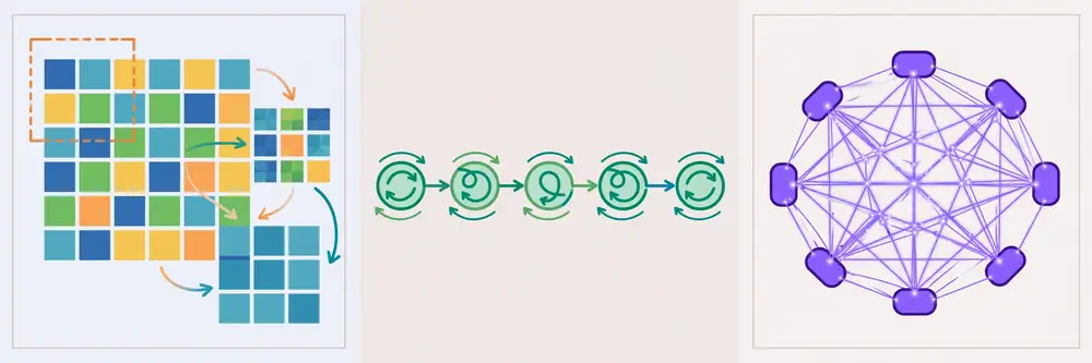
Two tokens with 2D query/key vectors. Queries Q = [[1, 0], [0, 1]]; Keys K = [[1, 0], [0, 1]] (token 1's key matches token 1's query, etc.). d = 2, √d ≈ 1.414.

Scores = QKᵀ/√d: - Token 1 vs keys: [1·1+0·0, 1·0+0·1]/1.414 = [0.707, 0] - Token 2 vs keys: [0, 0.707]

Softmax each row: softmax([0.707, 0]) = [e^0.707, e^0]/sum = [2.028, 1]/3.028 ≈ [0.670, 0.330]. Row 2 mirrors: [0.330, 0.670].

So token 1's output = 0.670·V₁ + 0.330·V₂ — it mostly takes its own value but mixes in a third of token 2's. With learned Q/K projections, these weights become the "it → dog" links. The whole mechanism is just similarity → softmax → weighted average, repeated at every layer.

What this means for your research

You probably won't train a Transformer from scratch — you'll fine-tune a pre-trained one (BERT for text classification, a vision Transformer for images), exactly the transfer-learning playbook from Chapter 8. The research contributions available to students: applying pre-trained Transformers to a new domain/language/task (low-resource languages are a real gap), comparing architectures, probing attention patterns, or making them smaller/faster (distillation, quantization). When you write it up, name the exact pre-trained checkpoint, the fine-tuning hyperparameters, and the maximum sequence length — reviewers will ask.

Positional encodings and residual connections, concretely

Two components deserve a closer look, because papers mention them in passing and beginners gloss over them.

Positional encodings. Self-attention is permutation-invariant: shuffle the tokens, and (without positions) the output shuffles identically — the model literally cannot tell word order. The original Transformer adds a fixed pattern of sine and cosine waves of different frequencies to each token embedding [5]: position p gets sin(p/10000^(2i/d)) in even dimensions, cos(...) in odd. Each position thus has a unique "fingerprint," and relative distances are encoded in phase differences the model can learn to read. Modern variants use learned position vectors or rotary embeddings instead — when a paper names one, it's a detail worth recording, since it affects maximum sequence length.

Residual connections + layer norm. Each sub-layer (attention, feedforward) is wrapped as: output = LayerNorm(x + Sublayer(x)). The addition is the residual highway from Chapter 2 — gradients flow straight back through the "+" even in a 96-layer model. LayerNorm rescales each token's vector to stable statistics, preventing the drift that deep stacks accumulate. Ablation studies consistently show Transformers train poorly without both; if your from-scratch Transformer won't converge, these are the first components to verify, not the attention math.

Vision Transformers and where Transformers struggle

Transformers escaped language: the Vision Transformer (ViT) chops an image into patches (e.g., 16×16), treats each patch as a "token," and applies the standard architecture — no convolution at all. With enough data it matches or beats CNNs, suggesting attention is a general-purpose relational engine, not a language-specific trick.

But be honest about weaknesses — reviewers will be. Transformers are data-hungry (weak inductive bias means they learn structure from examples rather than assuming it, unlike CNNs' built-in locality), quadratically expensive in sequence length, and their attention maps are suggestive but not faithful explanations. For small datasets, a CNN or LSTM often wins — "we used a Transformer" is not automatically the stronger paper; "we used the right tool for our data regime, with ablations" is.

The decoder and masked attention: how generation works

GPT-style models generate text one token at a time, and the mechanism is worth understanding because you'll use these models as research tools. During training, masked (causal) attention prevents each position from seeing future tokens — the attention mask sets future scores to −∞ before the softmax, so weights are exactly 0. The model thus learns "predict token t from tokens 1…t−1" at every position simultaneously.

At inference, generation is a loop: feed "The cat sat", predict the next-token distribution, sample "on", feed "The cat sat on", predict "the", and so on. Each step reuses cached keys/values (the KV-cache) so it doesn't recompute the whole past. Two inference knobs you'll meet in papers: temperature (Chapter 3's softmax dial — low = deterministic, high = creative) and top-k/top-p sampling (restrict sampling to the most probable tokens). When you evaluate LLM outputs for research, report these settings — they change results as much as the model choice.

The original 2017 Transformer was an encoder-decoder for translation [5]: the encoder reads the source sentence (bidirectional attention), and the decoder generates the target sentence one token at a time, attending both to its own past (masked self-attention) and to the encoder's output (cross-attention — queries from the decoder, keys/values from the encoder). If your task maps one sequence to another (translation, summarization, speech-to-text), this is the architecture shape to reach for; for classification or pure generation, the encoder-only or decoder-only variants suffice. Naming the variant correctly in your paper ("we fine-tune an encoder-only BERT-style model") prevents reviewer confusion.

Finally, a vocabulary note for reading papers: "self-attention" (within one sequence, as above), "cross-attention" (between two sequences, as in the decoder), and "multi-head attention" (several in parallel) are the three terms that cover nearly every mention. If you can explain those three sentences, you can follow any Transformer methods section.

For your research: Do not treat a Transformer as magic — Chapter 12 will show you how to describe it precisely (layers, heads, hidden size, checkpoint name). A common reviewer objection is "why a Transformer and not a simpler model?": answer with an ablation (LSTM vs. Transformer on your data) or a principled reason (long-range dependencies, pre-trained checkpoint availability). And remember the quadratic cost — if your sequences are very long (genomics, long documents), discuss how you handled it (truncation, sliding windows, efficient variants); ignoring it looks naive.

Key takeaways - Self-attention = queries matching keys → softmax weights → weighted sum of values; multi-head runs several in parallel. - Transformers beat RNNs via parallelism and direct long-range connections; cost is quadratic in sequence length. - Anatomy: attention → add&norm → feedforward → add&norm, stacked; residual connections and positional encodings are essential. - In practice: fine-tune pre-trained checkpoints; report the checkpoint, layers, heads, and sequence length.

---

Chapter 11: Practical Tips — Initialization, Normalization, Debugging Training

Theory tells you what should work. This chapter is about what to do when it doesn't — the craft knowledge that separates a researcher who trains models from one who only reads about them. Three topics cover most real failures: how weights start (initialization), what scale data enters at (normalization), and how to read the symptoms when training misbehaves (debugging).

Initialization: starting weights well

If all weights start at zero, every neuron in a layer learns identically — symmetry never breaks. If they start too large, activations saturate (sigmoid/tanh) or explode; too small, and signals vanish. The fix: random initialization with variance matched to the layer size and activation:

• Xavier/Glorot initialization (for sigmoid/tanh): draw weights from a distribution with variance 1/n_in, where n_in is the number of inputs to the neuron. Keeps signal variance stable across layers.
• He initialization (for ReLU): variance 2/n_in — the factor of 2 compensates for ReLU killing half the activations.

Frameworks do this by default when you create a layer [7][8] — but only if you use their layer constructors. Hand-rolled weight matrices with the wrong scale are a classic silent bug. Biases usually start at zero (safe, since weights break the symmetry).

Worked mini-example: a ReLU layer with n_in = 100 inputs. He says: std = √(2/100) ≈ 0.141. So initialize weights ~ Normal(0, 0.141²). If you instead used std = 1.0, pre-activations would have variance ~100× too large → massive z values → (for sigmoid) total saturation, or (for ReLU) exploding activations downstream. One number, enormous consequences.

Normalization: taming the inputs and the internals

Neural networks are scale-sensitive: a feature ranging 0–1000 dominates one ranging 0–1, and gradient descent struggles on such stretched landscapes.

• Input standardization: x′ = (x − μ)/σ per feature (mean 0, std 1), or min-max scaling to [0,1] / [−1,1]. Compute μ, σ on the training set only, then apply to validation/test. For images, per-channel normalization with dataset statistics is standard.
• Batch normalization: normalizes each layer's pre-activations within each mini-batch during training, then applies learned scale/shift. It stabilizes deep networks, permits higher learning rates, and slightly regularizes. Layer normalization does the same per-example (no batch dependence) — standard inside Transformers [5].

If your loss is NaN by epoch 2 or stuck from the start, unnormalized inputs are suspect #1.

Debugging: reading the symptoms

Keep this diagnostic table near your workstation:

Symptom	Likely cause	Fix to try
Loss = NaN / explodes	Learning rate too high; unnormalized inputs; division by zero in custom loss	Lower LR 10×; standardize inputs; add epsilon to logs
Loss flat from epoch 1	Dead ReLUs from bad init; saturated sigmoids; bug (labels shuffled, wrong loss)	Check init; verify forward pass by hand (Ch. 4); confirm loss matches task (Ch. 5)
Train loss falls, validation rises	Overfitting	More data/augmentation; dropout; weight decay; early stopping
Both losses high and flat	Model too small; LR too low; bad features	Bigger network; raise LR; check data quality
Loss oscillates wildly	Learning rate too high; batch too small	Lower LR; increase batch size
Great training, poor test, no validation gap seen	You tuned on the test set (or leaked it)	Lock the test set away; re-split properly

Two meta-habits: (1) Start tiny. Before the full run, overfit a single batch — a healthy network should drive one batch's loss to ~0. If it can't, something is broken (bug, not hyperparameters). (2) Change one thing at a time and log everything; otherwise you can't attribute improvements, and your paper's ablation table writes itself from the log.

Worked example: standardizing features by hand

Feature values (house sizes, m²): [80, 120, 100, 140, 60]. Mean μ = 500/5 = 100. Variance = [(−20)² + 20² + 0² + 40² + (−40)²]/5 = (400+400+0+1600+1600)/5 = 4000/5 = 800 → σ ≈ 28.28. Standardized: (80−100)/28.28 ≈ −0.707; (120−100)/28.28 ≈ 0.707; 0; 1.414; −1.414. Now the feature is centered at 0 with unit spread — gradient descent treats it fairly alongside your other features. In code this is one function call, but knowing the arithmetic means you can sanity-check any preprocessing pipeline.

Gradient checking: verifying your backprop

Frameworks compute gradients for you — but your custom loss or layer might feed them wrong inputs. Gradient checking verifies the backward pass against finite differences: for a weight w, compute [L(w+ε) − L(w−ε)] / 2ε with ε = 10⁻⁵ and compare to the framework's ∂L/∂w. They should agree to ~10⁻⁷ relative error. We did exactly this in Chapter 6's worked example (our −0.0936 vs. finite-difference −0.091).

Procedure: implement your model, run gradient check on a tiny version (few parameters, few examples), confirm agreement, then disable it — it's far too slow for real training. If it disagrees, the bug is in your forward math or in a non-differentiable operation you smuggled in. Run this check once per custom component; it has saved countless researchers from publishing results computed with broken gradients.

Pre-flight checklist before long training runs

GPU hours are expensive and queues are long. Before launching a multi-day run:

1. Overfit one batch — loss should approach ~0. If not, stop; something is broken.
2. Overfit a small subset (e.g., 500 examples) — checks the model can learn your data distribution at all.
3. Verify the full pipeline end-to-end on 2 epochs: data loading, forward, loss, backward, validation, checkpoint saving.
4. Check a validation curve on the short run — is it moving in the right direction?
5. Estimate total time (Chapter 7's arithmetic) and set up checkpointing + early stopping so an interrupted run isn't a lost run.
6. Fix your seeds and log everything — config file, git commit, dataset version.

Each step takes minutes and catches a different class of disaster. The researchers who "waste" an hour on this checklist are the ones whose week-long runs actually finish.

Reproducibility: seeds and determinism, concretely

"Mean ± std over seeds" deserves a concrete recipe, because vague claims here are a known credibility gap:

1. Fix all randomness sources: Python's random, NumPy, and the framework RNG (e.g., torch.manual_seed) — plus data-loader worker seeds, or shuffling differs per run.
2. Choose 3–5 seeds (42, 43, 44 is conventional; any fixed set works).
3. Train the full pipeline once per seed, changing nothing else.
4. Report mean ± standard deviation of your main metric. If a baseline scores 81.2 ± 1.5 and yours 82.0 ± 1.4, the "improvement" is noise — say so honestly, or run more seeds.

Full determinism (bit-identical reruns) additionally requires disabling nondeterministic GPU kernels, which slows training — most papers settle for fixed-seed statistics instead, and reviewers accept this. What they don't accept is a single lucky seed presented as the method's performance. Log the seeds in your config file from day one; reconstructing them after the fact is impossible.

Watching activations: the histogram habit

Beyond loss curves, peek at activation statistics every few epochs: the mean and spread of a few layers' outputs. Healthy signs: ReLU layers with 30–70% sparsity and pre-activation spreads in the single digits; batch-norm outputs near mean 0, std 1. Warning signs: activations stuck at 0 (dead layer — check init/LR), values exploding into the thousands (about to NaN — lower LR, check normalization), or a layer whose outputs never change across different inputs (it's being bypassed — check skip connections or a bug).

This takes five lines of logging code and catches an entire class of failures that loss curves reveal only late. In your paper's appendix or supplementary material, one such histogram figure ("activation distributions at epoch 1 vs. epoch 50") signals unusual training rigor to reviewers who know what to look for.

One last debugging ally: learning-curve shape. A healthy curve falls fast, then slowly, then plateaus. A curve that falls in sharp steps may indicate your learning-rate schedule is doing all the work (fine, but note it). A curve that plateaus high then suddenly drops suggests the optimizer escaped a plateau — consider a longer warmup next time. After a dozen runs you'll read these shapes like handwriting.

For your research: Reviewers increasingly expect a "training details" paragraph or table: initialization scheme, normalization, optimizer, learning rate + schedule, batch size, epochs/stopping rule, hardware, framework version, and random seeds. Seeds matter — report the mean ± std over 3–5 seeds, not a single lucky run; it is the cheapest credibility boost in experimental ML. And when a baseline "doesn't work," debug it with this chapter before claiming your method is better — nothing undermines a paper like a baseline that failed from a fixable training bug.

Key takeaways - Initialize with Xavier (tanh/sigmoid) or He (ReLU) variance scaling; never all-zeros. - Standardize inputs (train-set statistics only); consider batch/layer normalization inside deep networks. - Diagnose by symptom: NaN → LR/scale; flat → init/bug; val-rising → overfit; both-high → capacity/data. - Start tiny (overfit one batch), change one variable at a time, log everything, report mean ± std over seeds.

---

Chapter 12: From Theory to Paper — How to Describe Your Architecture in a Publication

You understand neural networks. Now you must communicate one — in a methods section that lets a stranger rebuild your model and trust your results. Reviewers reject papers not only for weak ideas but for undescribed methods. This chapter gives you the complete template: what to specify, how to draw it, and the sentences that signal competence.

The five things every architecture description needs

1. Structure: layer types, sizes, and order. "A 4-layer MLP: input(20) → FC(64, ReLU) → Dropout(0.3) → FC(32, ReLU) → FC(3, softmax)."
2. Parameter count: total trainable parameters (frameworks print this; report it). It contextualizes your model's size.
3. Training recipe: optimizer, learning rate + schedule, batch size, epochs/stopping rule, loss function, initialization, seeds — the full Chapter 7/11 checklist.
4. Data pipeline: dataset source, splits (with sizes), preprocessing/normalization, augmentation. Your model is meaningless without its data context.
5. Evaluation: metrics (accuracy, F1, MSE…), validation protocol, test procedure, and mean ± std over seeds.

Miss any one and a careful reviewer will ask for it in revision — or reject.

Drawing the diagram

Every neural-network paper has an architecture figure. Rules for a good one: left-to-right data flow, each block labeled with layer type and dimensions (e.g., "Conv 3×3, 64 filters → 112×112×64"), arrows showing tensor shapes changing, and no decorative 3D excess. Tools: simple PowerPoint/Keynote diagrams are fine; TikZ or PlotNeuralNet for LaTeX polish. The figure and the text must agree — a dimension mismatch between them is a red flag.

The hyperparameter table

A compact table is worth a page of prose:

Hyperparameter	Value
Architecture	1D-CNN: Conv(32, k=5)–ReLU–MaxPool–Conv(64, k=3)–ReLU–GlobalAvgPool–FC(3, softmax); 48,211 params
Optimizer	Adam, lr = 0.001, halve on plateau (patience 5)
Batch size / epochs	64 / early stopping (patience 10, max 100)
Loss	Categorical cross-entropy
Regularization	Dropout 0.3, weight decay 1e−4
Seeds	42, 43, 44 (mean ± std reported)
Framework / hardware	PyTorch 2.x [8], single NVIDIA GPU

A reviewer can replicate your work from this table plus the data description. That is the bar.

Ablations: proving each piece earns its place

An ablation study removes or swaps components and measures the damage: no dropout, ReLU→tanh, 2 layers vs. 4, with/without augmentation. Present as a small table with the full model on top. Ablations turn "we built a thing" into "we understand the thing" — they are among the highest-value pages in a student paper because they demonstrate scientific thinking, not just engineering.

Worked example: the methods paragraph, filled in

"We use a multilayer perceptron with two hidden layers (64 and 32 units, ReLU activations, He initialization) and a 3-way softmax output (12,739 trainable parameters). Inputs are standardized using training-set statistics. The network is trained with Adam (learning rate 10⁻³) minimizing categorical cross-entropy, batch size 64, with early stopping on validation loss (patience 10, maximum 100 epochs). We apply dropout (p = 0.3) after the first hidden layer. All results are mean ± standard deviation over three random seeds. The model was implemented in PyTorch [8]."

Every clause maps to this book: architecture (Ch. 2), activations + init (Ch. 3, 11), output + loss (Ch. 5), training loop (Ch. 7), regularization and seeds (Ch. 11). Write your paragraph by walking the same checklist — nothing missing, nothing vague.

Honest limitations (the section strong papers include)

State what your architecture cannot do: data regimes where it fails, compute costs, sensitivity to hyperparameters, and the Minsky-Papert-style boundary of its competence. "Our model requires ~2,000 labeled images; performance degrades below 500" is a limitation that increases trust. Reviewers are not looking for perfection; they are looking for authors who know exactly what they built.

Describing standard parts vs. novel contributions

Not every component deserves equal ink. A good methods section is selective:

• Standard parts (a ResNet encoder, Adam, cross-entropy): name them precisely with a citation and move on — "we use a ResNet-50 encoder [4] with ImageNet pre-training." Nobody needs the convolution equations re-derived.
• Modified parts (your changed loss, your added attention block): describe fully — equations, dimensions, motivation, and an ablation proving the change matters.
• Novel parts (your new architecture): describe exhaustively — diagram with dimensions, all equations, parameter counts, and ideally released code.

The common student error is inverted emphasis: three pages re-explaining backpropagation, one vague paragraph on the actual contribution. Your novelty gets the space; the textbook material gets a citation to [1] or [3].

Reviewer objections — and where this book answers them

Objection you'll hear	Your defense, grounded in this book
"Why this architecture?"	Match architecture to data structure (Ch. 8–10) + an ablation vs. a simpler baseline
"Why these hyperparameters?"	Report the search/selection procedure; show the key ablations (Ch. 7, 11)
"Is the improvement significant?"	Mean ± std over seeds; ideally a statistical test (Ch. 11)
"Can this be reproduced?"	Full recipe: architecture, training, data, seeds, code (Ch. 12 template)
"What are the limitations?"	State data requirements, failure modes, compute cost honestly (Ch. 12)
"Why not a Transformer / bigger model?"	Data-regime argument + ablation showing it didn't help (or wasn't feasible)

Keep this table in mind while writing — every row is a paragraph (or table) your paper should contain before the reviewer asks.

Example: describing the Chapter 8 CNN as a figure caption

Let's turn our traced CNN into publishable prose — the kind of caption + text pair reviewers expect:

Figure caption: "Proposed CNN architecture. Input: 64×64×3 images. Conv1 (32 filters, 3×3, stride 1, pad 1) → ReLU → MaxPool (2×2) → Conv2 (64 filters, 3×3) → ReLU → MaxPool (2×2) → Flatten (16,384) → FC(128, ReLU, dropout 0.5) → FC(10, softmax). Total: 2.1M trainable parameters."

Methods text: "We train with Adam (lr = 10⁻³, cosine decay over 50 epochs), batch size 64, categorical cross-entropy, and early stopping on validation loss (patience 8). Inputs are normalized per-channel using training-set statistics and augmented with random horizontal flips and ±10° rotations. Results are mean ± std over three seeds (42–44), implemented in PyTorch [8] on a single GPU."

Every number is checkable, every choice named, nothing decorative. Notice what isn't there: no re-derivation of convolution, no justification of Adam beyond naming it — standard parts get citations and one line each. Your novel contribution would then get its own paragraph with the same density. Write every architecture description to this standard and the methods section almost writes itself.

Code release checklist

Increasingly, reviewers (and journals) expect code. Before you link a repository, run this checklist:

1. One-command reproduction: a README that runs training and evaluation end-to-end (e.g., python train.py --config configs/final.yaml).
2. Pinned dependencies: requirements file with versions — "PyTorch 2.x" rots; "torch==2.3.1" reproduces.
3. Config files, not hardcoded values: every hyperparameter from your paper's table in one YAML/JSON.
4. Saved seeds and a results log: the exact seeds plus the raw per-seed metrics your table summarizes.
5. Pre-trained weights for your best model, with a load-and-predict script.
6. Data instructions: download links or collection procedure, preprocessing script, and the train/val/test split definition.

You don't need all six for a first submission, but items 1–3 are the difference between "code available" as a real claim and as decoration. A reproducible repository turns your paper from a report into a tool other researchers build on — which is how citations accumulate.

The abstract's one sentence

Your architecture also needs a one-sentence version for the abstract — the elevator pitch reviewers read first. Formula: "[Architecture] with [key property] for [task], achieving [metric]." Example: "We fine-tune a pre-trained ResNet-50 with a lightweight attention head for wheat disease classification, reaching 94.1 ± 0.8% accuracy on field images." Twelve words of method, one number, one dataset qualifier. If a reader can't grasp your approach from that sentence, the methods section has to work too hard. Draft this sentence before writing the full methods section — it forces you to decide what actually matters about your design.

For your research: Before submitting, run the "stranger test": give your methods section to a colleague and ask if they could reimplement the model without asking you anything. Every question they ask is a missing sentence. Then check reproducibility artifacts: fixed seeds, logged hyperparameters, saved model weights, and — increasingly expected — code. A paper whose architecture is fully specified, ablated, and honestly limited is publishable even when the accuracy gain is modest; a vague one is rejectable even when the numbers are good.

Key takeaways - Specify five things: structure, parameter count, training recipe, data pipeline, evaluation protocol. - Draw a clean dimension-labeled diagram; make figure and text agree. - Tabulate hyperparameters; ablate every non-obvious choice. - Report mean ± std over seeds; state limitations honestly — precision builds more trust than big numbers.

---

References

[1] I. Goodfellow, Y. Bengio, and A. Courville, Deep Learning. Cambridge, MA, USA: MIT Press, 2016.

[2] F. Chollet, Deep Learning with Python, 2nd ed. Shelter Island, NY, USA: Manning, 2021.

[3] Y. LeCun, Y. Bengio, and G. Hinton, "Deep learning," Nature, vol. 521, no. 7553, pp. 436–444, May 2015.

[4] A. Krizhevsky, I. Sutskever, and G. E. Hinton, "ImageNet classification with deep convolutional neural networks," in Proc. Adv. Neural Inf. Process. Syst., vol. 25, 2012.

[5] A. Vaswani et al., "Attention is all you need," in Proc. Adv. Neural Inf. Process. Syst., vol. 30, 2017.

[6] C. M. Bishop, Pattern Recognition and Machine Learning. New York, NY, USA: Springer, 2006.

[7] A. Géron, Hands-On Machine Learning with Scikit-Learn, Keras, and TensorFlow, 2nd ed. Sebastopol, CA, USA: O'Reilly Media, 2019.

[8] A. Paszke et al., "PyTorch: An imperative style, high-performance deep learning library," in Proc. Adv. Neural Inf. Process. Syst., vol. 32, 2019.

[9] S. Russell and P. Norvig, Artificial Intelligence: A Modern Approach, 4th ed. Hoboken, NY, USA: Pearson, 2020.

---

Glossary

• Activation function — A nonlinear function applied to each neuron's weighted sum (e.g., ReLU, sigmoid); what makes deep networks more powerful than linear models.
• Attention — A mechanism that lets each sequence position weigh the relevance of all other positions; the core of the Transformer.
• Backpropagation — The chain-rule algorithm that efficiently computes the gradient of the loss with respect to every weight, working backwards through the network.
• Batch — The subset of training examples used for a single gradient update.
• Batch normalization — A technique that normalizes each layer's activations within a mini-batch to stabilize and speed up training.
• Bias — A learnable offset added to a neuron's weighted sum before the activation function.
• CNN (convolutional neural network) — A network using sliding filters to detect local patterns; the standard architecture for image data.
• Cross-entropy — The standard loss function for classification; heavily penalizes confident wrong predictions.
• Dropout — A regularization technique that randomly deactivates neurons during training to reduce overfitting.
• Epoch — One complete pass through the entire training set.
• Gradient descent — The optimization procedure that updates weights a small step opposite the loss gradient.
• Hidden layer — Any layer between the input and output layers; where intermediate representations are learned.
• Learning rate — The step-size hyperparameter scaling each gradient-descent update.
• Loss function — A single number measuring prediction error (e.g., MSE, cross-entropy); the quantity training minimizes.
• LSTM — A recurrent network variant with gated memory cells that preserve information over long sequences.
• MLP (multilayer perceptron) — A feedforward network with one or more hidden layers; the classic fully connected architecture.
• MSE (mean squared error) — The standard loss for regression: the average of squared prediction errors.
• Overfitting — When a model memorizes training data and performs poorly on new data.
• Perceptron — The earliest trainable artificial neuron (1958); learns a linear decision boundary.
• ReLU — Rectified linear unit, max(0, z); the most common hidden-layer activation in modern networks.
• RNN (recurrent neural network) — A network that processes sequences by passing a hidden state from step to step.
• Softmax — A function converting raw scores into a probability distribution over classes.
• Transformer — An architecture built on self-attention instead of recurrence; the basis of modern language models.
• Vanishing gradient — The shrinking of gradients in deep or long-unrolled networks, which stalls learning in early layers.
• Weight — A learnable parameter controlling how strongly one neuron's output influences the next.

---

Practice Exercises

1. Perceptron by hand. Using the perceptron learning rule with learning rate η = 1, starting from w = [0, 0], b = 0, train on the AND function ((0,0)→0, (0,1)→0, (1,0)→0, (1,1)→1). Show each update until all four examples are classified correctly, and write down the final decision boundary equation.
2. XOR impossibility. Prove (with a sketch and a few lines of algebra) that no single straight line can separate the XOR points {(0,0), (1,1)} from {(0,1), (1,0)}. Then verify the Chapter 2 network computes NAND instead of XOR if you change only the output bias — what bias value does that?
3. Activation arithmetic. Compute σ(z), tanh(z), ReLU(z) and their derivatives at z ∈ {−3, −1, 1, 3}. At which of these points is the sigmoid derivative below 0.05? What does that imply for a 6-layer sigmoid network?
4. Forward pass. For the Chapter 4 network (W⁽¹⁾ = [[0.8, −0.4],[0.2, 0.9]], b⁽¹⁾ = [0.1, −0.2], W⁽²⁾ = [[0.7, −0.6]], b⁽²⁾ = [0.0]), compute the full forward pass for x = [1.0, 1.0]. Which hidden neurons are active?
5. Loss computation. A 3-class model outputs probabilities [0.2, 0.5, 0.3] for a sample whose true class is 2 (one-hot [0,0,1]). Compute the categorical cross-entropy loss. Then compute the MSE loss for predictions [2.0, 4.0] against targets [3.0, 3.0]. Which loss would you use for a medical-diagnosis classifier, and why?
6. Backpropagation by hand. A single sigmoid neuron has w = 1.0, b = 0, input x = 0.5, target y = 0, and MSE loss L = ½(ŷ − y)². Compute ∂L/∂w and ∂L/∂b exactly as in Chapter 6, verify with a finite-difference check (Δw = 0.01), then perform one gradient-descent update with η = 2.0 and confirm the loss decreased.
7. Training arithmetic. You have 40,000 training examples, batch size 128, and each iteration takes 0.15 s. How many iterations per epoch? How long do 25 epochs take? If validation loss rises at epoch 18 while training loss keeps falling, what do you do, and what do you report?
8. Convolution by hand. Convolve the 3×3 image [[2,0,1],[1,3,2],[0,1,4]] with the 2×2 filter [[1,−1],[0,1]] (stride 1, no padding). Apply ReLU, then 2×2 max-pooling. How many learnable parameters does a convolutional layer with 16 such filters have (including biases)?
9. RNN unrolling. Using h_t = tanh(0.5·x_t + 0.9·h_{t−1}), h_0 = 0, compute h_1, h_2, h_3 for x = [2.0, −1.0, 0.5]. Then explain in two sentences why the contribution of x_1 to h_3 is already fading, and name the architecture that fixes this.
10. Mini research task. Pick a small public dataset (e.g., Iris or MNIST). Train an MLP with two different activations (ReLU vs. tanh) and two depths (1 vs. 3 hidden layers) — four runs, three seeds each. Write a one-page methods section following Chapter 12's template (architecture, hyperparameter table, mean ± std results, one ablation sentence, two limitations). This is the skeleton of your first publishable experiment.

---

End of Book 7. Next: Book 8 — Gradient Descent Explained Simply.