Gradient Descent Explained Simply

Book 8 of 10 — AstolixGen Learning Series (Detailed Edition) · For researcher and publication students

---

About This Book

Almost every machine learning model you will ever train is trained by some version of one algorithm: gradient descent. Whether you are fitting a regression line to survey data, fine-tuning a transformer for Urdu text, or training a small neural network for crop-disease detection, the same loop runs underneath: measure how wrong the model is, compute the gradient, and take a small step downhill. This book unpacks that loop completely — the intuition, the mathematics you actually need, the variants, the hyperparameters, and the failure modes.

This book is written for MS/PhD students and early researchers who want more than "just call optimizer.step()." You will be able to hand-compute gradient descent steps, choose an optimizer and learning rate with reasons you can defend, diagnose a stuck training run, and — critically — report your optimization setup in a paper so that a reviewer and a reader can reproduce your work.

Learning objectives: - Explain what optimization means in machine learning and what a loss function measures - Define the gradient and explain why stepping opposite to it reduces the loss - Carry out batch, stochastic, and mini-batch gradient descent by hand on small problems - Compare learning rates numerically and explain why too large diverges and too small crawls - Explain momentum and Nesterov acceleration and show how they speed convergence - Compute AdaGrad, RMSprop, and Adam updates step by step, including Adam's bias correction - Design learning rate schedules and warmup phases, and follow a practical tuning workflow from defaults to multi-seed final runs - Diagnose plateaus, ravines, saddle points, and other convergence problems, and apply fixes - Describe second-order methods honestly: what they offer and why deep learning rarely uses them - Write a reproducible optimization section for a research paper that satisfies reviewers

---

Learning Dashboard

Concept	Definition (one line)	Example	Use in research
Optimization	Finding the parameters that minimize (or maximize) an objective function	Fitting a line to house-price data by minimizing error	Every model you train is an optimization problem; name your objective explicitly in your paper
Loss function	A number measuring how wrong the model's predictions are	Mean squared error on house prices	Choose a loss matched to your task; reviewers judge whether it fits
Parameter (weight)	A tunable number inside the model, adjusted during training	Slope and intercept of the fitted line	Report your model's parameter count; it speaks to complexity and compute cost
Gradient	The vector of partial derivatives; points in the direction of steepest increase of the loss	Slope of the loss curve at the current weights	Understanding gradients lets you diagnose why training is stuck
Learning rate	The step-size multiplier on the negative gradient	η = 0.01 versus η = 1.0	Report the exact value and schedule; it is the first thing a reviewer checks for reproducibility
Batch gradient descent	Uses the entire dataset for every single update	10,000 images averaged into one gradient	Stable updates; a useful baseline in small-data experiments
Stochastic gradient descent	Uses one randomly chosen example per update	One image per update step	Fast steps on large data; the noise can help escape sharp minima
Mini-batch gradient descent	Uses a small random subset per update	32 images per update step	The standard choice; balances stability, speed, and GPU efficiency
Momentum	Carries a running average of past gradients to accelerate consistent directions	A ball rolling downhill gaining speed	Speeds training on ravines; the standard add-on to SGD
Nesterov momentum	Momentum that first looks ahead, then computes the gradient	Steering before braking	Often converges faster than plain momentum; used in many baselines
AdaGrad	Scales each parameter's learning rate by its accumulated past gradients	Rare word features get bigger steps	Good for sparse data (e.g., text); the rate can decay too fast
RMSprop	AdaGrad with an exponentially decaying average of squared gradients	Fixes AdaGrad's rapid decay	Strong default for recurrent networks and non-stationary problems
Adam	Momentum plus adaptive per-parameter rates, with bias correction	The default optimizer in most deep learning papers	Start here; report β₁, β₂, and ε, not just the word "Adam"
Learning rate schedule	A rule that changes the learning rate during training	Halve the rate every 10 epochs	Schedules squeeze out final accuracy; report the exact rule
Warmup	Starting with a tiny learning rate that ramps up over early epochs	0 → 0.01 over the first 5 epochs	Stabilizes large-batch training of transformers and deep nets
Local minimum	A point lower than everything nearby, but not necessarily the global best	A small dip in the loss landscape	In deep networks, saddle points worry researchers more than local minima
Saddle point	Gradient is zero but the point is a minimum in some directions and a maximum in others	A mountain pass	The main convergence obstacle in high dimensions; noise and momentum help
Second-order method	Uses curvature (the Hessian matrix) in addition to the gradient	Newton's method converging in one step on a quadratic	Rarely used in deep learning, but relevant for small models and theory papers

Roadmap of chapter connections. Chapter 1 frames training as optimization; Chapter 2 gives you the gradient, the compass for the whole book. Chapters 3 and 4 turn the compass into three algorithms — batch, stochastic, mini-batch — and Chapter 5 tunes the most important dial, the learning rate. Chapters 6 and 7 add intelligence to the steps (momentum, then adaptive methods), while Chapter 8 controls the dial over time (schedules and warmup). Chapter 9 assembles everything into a tuning workflow you can follow on Monday morning. Chapter 10 is the troubleshooting guide for when the workflow fails, Chapter 11 looks honestly at the more expensive alternatives, and Chapter 12 shows you how to write all of this up so your paper is reproducible.

---

Chapter 1: Optimization in Machine Learning — The Big Picture

Training is just optimization wearing a lab coat

When you "train" a machine learning model, you are solving an optimization problem. The model has knobs — parameters, usually called weights — and the data tells you how good each knob setting is through a single number: the loss. Training means turning the knobs until the loss is as small as possible. That is all. Everything else in this book is detail about how to turn the knobs well.

This framing matters for your research because every claim you make about a model — "it achieves 94% accuracy," "it trains twice as fast" — is a claim about an optimization outcome. If you cannot describe what was optimized, how, and how well, your results are not interpretable.

The three ingredients

Every optimization problem in machine learning has the same three ingredients:

1. Parameters (θ). The numbers the algorithm is allowed to change. In a line model y = wx + b, the parameters are w and b. In a neural network, they are millions of weights and biases. We write them as a vector θ to keep things general.

2. A loss function L(θ). A formula that takes a parameter setting and returns one number: how bad the model is. Also called the objective function or cost function. Examples: mean squared error for regression, cross-entropy for classification. The loss is computed on the training data.

3. An optimizer. The procedure that picks new parameter values, over and over, to drive the loss down. Gradient descent and its variants are the optimizers this book covers.

Notice what is not in the list: accuracy. Accuracy is what you care about, but optimizers need a smooth, differentiable number to work with, and accuracy is a staircase — it jumps in discrete steps, so it has no useful gradient. This is why you minimize cross-entropy loss while reporting accuracy. They usually move together, but they are different instruments: the loss is the steering wheel, accuracy is the dashboard.

A concrete picture: fitting a line

Suppose you want to predict house prices from area. You choose the model y = wx (price proportional to area, no intercept, to keep it simple) and the mean squared error loss:

L(w) = (1/n) Σ (wxᵢ − yᵢ)²

With three houses — (100 m², 100), (200 m², 200), (300 m², 300) in some units — the loss becomes L(w) = (28/9)(w − 1)², which is a perfect U-shape (a parabola) with its bottom at w = 1. Training is now a one-dimensional treasure hunt: find the w that sits at the bottom of the U.

Worked example: evaluating candidate parameters by hand

Take L(w) = (w − 3)², a parabola bottoming out at w = 3. Before we learn any algorithm, let's just evaluate it at a few guesses, the way a brute-force search would:

• w = 0 → L = (0 − 3)² = 9
• w = 2 → L = (2 − 3)² = 1
• w = 3 → L = 0 ← the minimum
• w = 4 → L = (4 − 3)² = 1

Two observations that will matter later. First, the loss surface has a shape — here a bowl — and the optimizer's job is to walk to the bottom of it. Second, brute-force guessing works in one dimension but is hopeless with a million parameters: you cannot grid-search a million-dimensional space. You need a guided walk, one that uses local information about which direction is downhill. That guidance is the gradient, the subject of Chapter 2.

Why optimization is hard in deep learning

In the examples above, the loss surface was a friendly bowl. Real neural network loss surfaces are not. They live in millions of dimensions, they are non-convex (full of hills, valleys, and flat plains), and you cannot visualize them. Three facts keep researchers humble:

• There is no known efficient algorithm that guarantees finding the global minimum of a deep network's loss. We settle for good local solutions.
• The loss you minimize (training loss) is not quite the thing you care about (test performance). Optimize too aggressively and you overfit — you memorize the training data instead of learning the pattern.
• Computing the exact gradient over the full dataset can be enormously expensive, which is why we use approximations (Chapter 4).

None of this stops gradient descent from working remarkably well in practice. But it explains why the details — learning rates, batch sizes, schedules — matter so much, and why papers report them.

The vocabulary reviewers expect

When you write a paper, use these terms precisely. Training is the whole process. An epoch is one full pass over the training data. An iteration (or step) is one parameter update. Convergence means the parameters have settled — the loss is no longer decreasing meaningfully. A hyperparameter is a setting you choose before training (learning rate, batch size) as opposed to a parameter, which the optimizer learns. Mixing these up in a paper signals inexperience to a reviewer, so get them straight now.

Convex vs. non-convex: why some problems are easy

Not all loss surfaces are equally hostile. A convex function is a bowl in the strong sense: the line segment between any two points on its graph lies above the graph. The function x² is convex; so is |x|; and so is the mean-squared-error loss of linear regression. Convexity buys a powerful guarantee: every local minimum is the global minimum. Gradient descent cannot get trapped in a second-rate dip because there are no second-rate dips — wherever the gradient reaches zero, you have found the best possible answer.

This is why classical machine learning (linear regression, logistic regression, support vector machines) comes with convergence guarantees: with an appropriate learning rate, batch gradient descent will find the global minimum. If your research uses a convex model, say so in the paper — it upgrades your claims from "we found a good solution" to "we found the optimal solution," and reviewers respect the distinction.

Deep networks are non-convex: their loss surfaces have many minima of different depths, plus saddle points (Chapter 10). No efficient algorithm guarantees the global minimum. Here is the signature of non-convexity, computed by hand. Take f(x) = x⁴ − 4x². Its derivative is f′(x) = 4x³ − 8x = 4x(x² − 2), which is zero at x = 0 and x = ±√2 ≈ ±1.414. The points ±1.414 are two equally deep minima (f = −4); x = 0 is a local maximum sitting between them.

Run gradient descent with η = 0.1 from x₀ = 1: f′(1) = −4, so x₁ = 1 + 0.4 = 1.4. Then f′(1.4) = 4(1.4)(1.96 − 2) = 5.6 × (−0.04) = −0.224, and x₂ = 1.4 + 0.0224 = 1.4224 — settling toward +1.414. Now start instead at x₀ = −1: f′(−1) = 4, x₁ = −1.4, and the walk converges to −1.414. Same algorithm, same function, different starting point, different minimum. That cannot happen with a convex function.

One comforting fact for deep learning: modern networks are so overparameterized that most of their local minima turn out to be roughly equally good (Chapter 10). So the practical takeaway is calibration, not despair: for non-convex deep learning, stop asking "did I find the global minimum?" and start asking "did I find a minimum that generalizes well?" And fix your random seeds (Chapter 12) — since the starting point partly decides the destination, an honest paper reports results across several of them.

The optimization–generalization gap

Here is a subtlety that trips up many beginners: the optimizer minimizes the loss on the training data, but you care about performance on unseen data. These are different objectives, and driving the first to zero does not guarantee the second. A model that memorizes every training example — loss exactly zero — can fail completely on new inputs. This is overfitting, and it is why optimization success and research success are not the same thing.

The standard defense is a three-way data split: train on the training set, make decisions (early stopping, hyperparameter choices) on the validation set, and report final numbers on the test set — which you touch exactly once, at the end. Think of it as three roles: the training set teaches, the validation set advises, the test set judges. A classic symptom of overfitting is a training loss that keeps falling while the validation loss starts rising — the model is still "optimizing" but no longer learning anything useful. Early stopping (Chapter 9) halts training at the validation minimum.

For your research mindset, remember: this book teaches you to minimize loss efficiently, but a good researcher always asks "loss on which data?" An optimizer can only descend the surface you give it. Choosing the right surface — the right loss, the right data split, the right stopping point — is where machine learning becomes a science rather than an exercise in curve-fitting.

For your research: In your paper's methodology section, state the optimization problem in one sentence: "We minimize the cross-entropy loss over the network parameters θ using mini-batch gradient descent." That single sentence tells the reader the loss, the parameters, and the optimizer. Then Chapter 12 of this book will show you the full reporting checklist. Start collecting these details from day one of your experiments — reconstructing them after submission is painful and error-prone.

Key takeaways - Training = choosing parameters θ to minimize a loss function L(θ); everything else is technique. - The loss is the steering wheel (smooth, differentiable); accuracy is the dashboard (what you report). - Brute-force search cannot work in high dimensions; you need gradient-guided steps. - Epoch, iteration, convergence, hyperparameter vs. parameter — use these terms exactly. - Deep learning optimization has no global-minimum guarantees; we aim for good, generalizing solutions.

---

Chapter 2: Gradients, Intuitively — Slopes, Directions, and Why They Matter

The slope is the whole trick

Stand on a hillside in fog. You want to reach the valley floor but cannot see more than a meter ahead. What do you do? You feel the slope under your feet and walk downhill. That is gradient descent. The gradient is the mathematical version of "feeling the slope": at any point, it tells you which direction is steepest uphill and how steep it is. Walk the opposite way and you go downhill — guaranteed, at least for a small step.

Formally, for a function of one variable f(x), the gradient is just the derivative f′(x): the slope of the curve at x. For a function of many variables L(θ₁, θ₂, …, θₙ), the gradient ∇L is the vector of partial derivatives (∂L/∂θ₁, …, ∂L/∂θₙ). Each entry says: "if you nudge this one parameter a tiny bit, holding the others fixed, the loss changes by this much per unit nudge."

Sign and size: reading a gradient

A gradient carries two pieces of information, and both matter:

• Sign (direction). A positive derivative means the function is increasing as you move right — so to decrease it, move left. A negative derivative means move right. The update rule "step = −(learning rate) × gradient" is just this: go against the sign.
• Magnitude (steepness). A large gradient means the slope is steep — you are far from flat ground, and (with a fixed learning rate) you will take a large step. A tiny gradient means you are on nearly flat ground, so steps become tiny. This is elegant: the algorithm automatically takes big strides on steep slopes and tiptoes near the bottom.

This self-adjusting step size is why plain gradient descent works at all, and it is also why it can be slow near the minimum (Chapter 10).

Where do gradients come from in practice?

You will almost never compute gradients by hand for a real model. The chain rule from calculus, applied mechanically through a computation graph, gives every partial derivative — this automation is called backpropagation, and frameworks like PyTorch and TensorFlow do it for you. But "the framework handles it" is not an excuse to skip understanding: when training fails, the gradient is the first diagnostic. "Vanishing gradients" (gradients near zero in early layers) and "exploding gradients" (enormous gradients) are among the most common failure modes in deep learning, and you cannot fix what you cannot picture.

Worked example: one gradient step, fully by hand

Take f(x) = x², the simplest bowl, with its minimum at x = 0. The derivative is f′(x) = 2x.

Start at x = 4. The gradient there is f′(4) = 8. Reading it: positive and large — the function is rising steeply to the right, so we should move left, and by a good amount.

Apply one gradient descent step with learning rate η = 0.1:

x_new = x − η · f′(x) = 4 − 0.1 × 8 = 4 − 0.8 = 3.2

Check the result: f(4) = 16, f(3.2) = 10.24. The loss fell from 16 to 10.24 in a single step. The negative gradient pointed downhill, and following it worked.

Now read the new gradient: f′(3.2) = 6.4. Still positive, so keep moving left — but smaller than 8, so the next step (0.64) will be smaller than the first (0.8). You can see the self-adjusting behavior already: as x approaches 0, the gradient shrinks toward 0 and the steps shrink with it, so the walk naturally slows down as it arrives. That is the entire mechanism of gradient descent, and everything in the rest of this book is a refinement of it.

The multi-dimensional picture

With two parameters, the loss is a surface — a landscape with hills and valleys — and the gradient at a point is an arrow lying on that landscape, pointing in the direction of steepest ascent. The update θ ← θ − η∇L(θ) moves against the arrow. With a million parameters you cannot draw the landscape, but the arithmetic is identical: each parameter gets nudged opposite its partial derivative. One subtlety worth knowing: the negative gradient is the steepest descent direction only for infinitesimally small steps; for any finite step it is merely a good downhill direction. That gap between "steepest" and "good" is where learning rates, momentum, and curvature all live.

Partial derivatives: the gradient with more than one parameter

In one dimension the gradient is a single slope. With two parameters — say a line model y = wx + b with loss L(w, b) = (w − 3)² + (b + 1)², whose minimum sits at w = 3, b = −1 — the gradient is a vector of two partial derivatives: ∂L/∂w = 2(w − 3) and ∂L/∂b = 2(b + 1). Each partial derivative asks one question: "holding the other parameter fixed, how fast does the loss change if I nudge this one?"

Evaluate at (w, b) = (0, 0): ∂L/∂w = −6, ∂L/∂b = 2, so ∇L = (−6, 2). Reading it: increasing w decreases the loss fast (negative slope — move w up); increasing b increases the loss (positive slope — move b down). One gradient descent step with η = 0.1 updates both simultaneously: w₁ = 0 − 0.1 × (−6) = 0.6; b₁ = 0 − 0.1 × 2 = −0.2.

Check the result: L(0, 0) = 9 + 1 = 10. L(0.6, −0.2) = (0.6 − 3)² + (−0.2 + 1)² = 5.76 + 0.64 = 6.4. Down from 10 to 6.4 in a single step, with each parameter walking its own downhill direction at its own pace — w moved 0.6 because its slope was steep, b moved only 0.2 because its slope was gentle.

That is the whole secret of high-dimensional optimization: nothing conceptually new happens at a million parameters. The gradient is a million-entry vector, each entry is one parameter's private slope, and the update nudges every parameter opposite its own slope in a single vector operation. You cannot draw the million-dimensional landscape, but you do not need to — the arithmetic is identical to the two-parameter case above, just longer. Frameworks compute all million partial derivatives in one backward pass, which is why backpropagation was such a breakthrough. And when Chapter 7 gives each parameter its own learning rate, it is simply letting each of these million private slopes set its own pace.

Numerical gradients: the debugging tool

Analytic gradients (from calculus or backpropagation) are fast but bug-prone — one wrong sign in a hand-derived gradient and training silently fails. Numerical gradients estimate the slope directly from function values using finite differences:

f′(x) ≈ (f(x + h) − f(x − h)) / (2h), with h tiny (e.g., 0.001)

Test it on f(x) = x² at x = 4, where the true derivative is 8: f(4.001) = 16.008001, f(3.999) = 15.992001. Difference: 0.016; divided by 0.002 → 8.0. Matches exactly (to rounding). This technique, called gradient checking, is how you verify a backpropagation implementation: compare its analytic gradients against numerical estimates on a tiny model. If they agree to ~10⁻⁵, your backward pass is correct.

Why not always use numerical gradients? Cost: each partial derivative needs two function evaluations, so a million-parameter model needs two million forward passes per gradient — absurd when backpropagation does it in one. Numerical gradients are a diagnostic instrument, not an engine: use them once, on a small model, to certify your gradients, then switch them off. Every deep learning framework's test suite does exactly this, and so should you whenever you implement a custom layer or loss.

A note on notation

Papers and textbooks use a compact notation that is worth learning early. Parameters are usually written as a vector θ (theta), the loss as L(θ) or J(θ), the gradient as ∇L(θ) (read "nabla L" or "grad L"), and the learning rate as η (eta) or α (alpha). The update θ ← θ − η∇L(θ) is read as "theta gets theta minus eta times the gradient of L." Superscripts like θ⁽ᵗ⁾ sometimes denote the parameters at step t. None of this is difficult — it is just shorthand — but fluency with it lets you read any optimization paper's method section without friction. When you write your own paper, define your symbols once ("we denote the parameters by θ ∈ ℝᵈ") and then use them consistently; reviewers notice sloppy or shifting notation.

For your research: When you read that a paper "trains with backpropagation," translate it: backpropagation computes the gradient, and an optimizer (covered in Chapters 3–7) uses it to update the parameters. In your own writing, never say "we trained using backpropagation" as if backpropagation were the optimizer — it is the gradient computer. Name the optimizer separately (e.g., "gradients were computed by backpropagation; parameters were updated with Adam"). Reviewers notice this distinction.

Key takeaways - The gradient = the slope (derivative) in 1-D, the vector of partial derivatives in n-D; it points steepest uphill. - Step = −η × gradient: the sign picks the downhill direction, the magnitude scales the stride. - Steps shrink automatically near the minimum because the gradient shrinks — a built-in braking system. - Backpropagation computes gradients; the optimizer decides the steps. They are different jobs. - Vanishing and exploding gradients are the classic gradient pathologies to watch for.

---

Chapter 3: Batch Gradient Descent, Step by Step

The honest, full-data algorithm

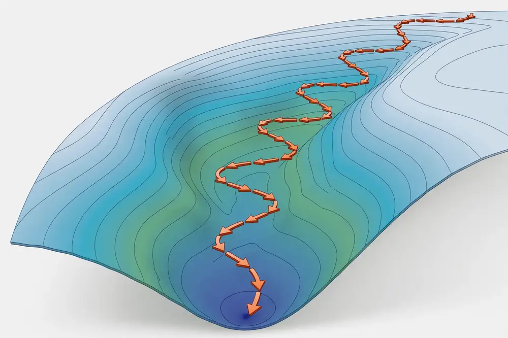
Batch gradient descent (often just called "gradient descent") is the textbook version: compute the gradient of the loss using every single training example, then take one step. Repeat until the loss stops improving. There is no randomness, no approximation — each step follows the true downhill direction of the training loss.

The update rule for parameters θ, learning rate η, and a dataset of n examples is:

θ ← θ − η · (1/n) Σᵢ ∇Lᵢ(θ)

where Lᵢ is the loss on example i. The (1/n) averaging keeps the gradient's scale independent of dataset size, so the same learning rate behaves similarly whether you have a hundred examples or a hundred thousand.

Why it is beautiful and why it is slow

Batch gradient descent has one great virtue: every step is trustworthy. Because the gradient is exact, the loss decreases monotonically on well-behaved problems, and the algorithm's behavior is deterministic — run it twice, get the same trajectory. That determinism makes it wonderful for teaching, debugging, and small research datasets.

Its flaw is cost. If you have a million training examples, each single step requires a million forward-backward passes. You might take only a handful of steps per hour. Worse, much of that computation is redundant: after seeing 10,000 examples, the gradient direction barely changes, yet you keep paying for the remaining 990,000. This inefficiency is what stochastic methods (Chapter 4) fix.

The algorithm, spelled out

1. Initialize the parameters θ (usually small random values; zeros can cause symmetry problems in neural networks).
2. Compute the loss and its gradient averaged over the entire training set.
3. Update: θ ← θ − η∇L(θ).
4. Repeat steps 2–3 until the loss stops decreasing (convergence) or you run out of patience (a fixed number of epochs).

That is the whole algorithm. Three lines of arithmetic, repeated.

Worked example: fitting a line with three points, by hand

Data: (x, y) = (1, 1), (2, 2), (3, 3). Model: y = wx (one parameter, no intercept — the true answer is clearly w = 1). Loss: mean squared error,

L(w) = (1/3)[(w·1 − 1)² + (w·2 − 2)² + (w·3 − 3)²] = (28/9)(w − 1)².

Differentiate (or trust the algebra): dL/dw = (2/3)Σ(wxᵢ − yᵢ)xᵢ = (28/3)(w − 1).

Setup: start w₀ = 0, learning rate η = 0.05.

Step 1. Gradient at w₀ = 0: (28/3)(0 − 1) = −28/3 ≈ −9.333. Negative → move right (increase w). w₁ = 0 − 0.05 × (−9.333) = 0.4667. Loss check: L(0) = 28/9 ≈ 3.111; L(0.4667) = (28/9)(0.4667 − 1)² = 3.111 × 0.2844 ≈ 0.885. Down from 3.111 to 0.885 — a real improvement.

Step 2. Gradient at w₁ = 0.4667: (28/3)(0.4667 − 1) = 9.333 × (−0.5333) ≈ −4.978. w₂ = 0.4667 − 0.05 × (−4.978) = 0.4667 + 0.2489 = 0.7156. Loss: L(0.7156) = 3.111 × (0.7156 − 1)² = 3.111 × 0.0809 ≈ 0.252.

Step 3. Gradient at w₂: 9.333 × (0.7156 − 1) ≈ −2.654. w₃ = 0.7156 + 0.05 × 2.654 = 0.8483. Loss: L ≈ 3.111 × (0.1517)² ≈ 0.0716.

Trajectory: w: 0 → 0.4667 → 0.7156 → 0.8483 → … → 1. Loss: 3.111 → 0.885 → 0.252 → 0.072 → … → 0. Each step uses all three points, each step is deterministic, and the loss falls smoothly. This is batch gradient descent working exactly as advertised.

Convergence: when do you stop?

In theory, you stop when the gradient is (near) zero. In practice, you stop when the loss stops improving by a meaningful amount — say, less than 0.001 change over several epochs — or when a fixed epoch budget is spent, or when validation performance starts degrading (early stopping, Chapter 9). For convex problems like linear regression, batch gradient descent with a sensible learning rate is guaranteed to converge to the global minimum; for deep networks, it converges to some minimum, and which one depends on initialization and the learning rate.

How fast does batch GD converge? The contraction factor

Look again at this chapter's trajectory: 0 → 0.4667 → 0.7156 → 0.8483, homing in on w = 1. There is hidden clockwork here. The update was w ← w − η·(28/3)(w − 1). Subtract 1 from both sides and factor: (w − 1) ← (w − 1)·(1 − 28η/3). The error (w − 1) is multiplied by a constant factor every step. With η = 0.05, that factor is 1 − 28×0.05/3 = 1 − 0.4667 = 0.5333.

Verify against the trajectory: error at w₀ is −1; ×0.5333 → −0.5333 (w₁ = 0.4667 ✓); ×0.5333 → −0.2844 (w₂ = 0.7156 ✓); ×0.5333 → −0.1517 (w₃ = 0.8483 ✓). Every step shrinks the remaining error to 53% of its previous value. This is called linear convergence, and it is the typical speed of gradient descent on well-behaved convex problems: steady, geometric, predictable.

Now watch the factor as η grows. With η = 0.1 the factor is 1 − 0.9333 = 0.0667: the error nearly vanishes each step — dramatically faster. With η = 0.107 the factor is ≈ 0: one-step convergence, a lucky strike resembling Newton's method (Chapter 11). With η = 0.3 the factor is 1 − 2.8 = −1.8: the error grows 1.8× per step with alternating sign — divergence, exactly the explosion from Chapter 5.

So the learning rate does not just scale steps; it sets the contraction factor, and there is a hard wall where the factor's magnitude exceeds 1. Bigger η means faster convergence right up to the wall — which is why tuning the learning rate (Chapter 9) is really a search for the largest stable η. On convex problems the wall sits at η < 2/L, where L is the steepest curvature of the loss; here the curvature is 28/3 ≈ 9.33, giving η < 0.214 — consistent with η = 0.3 diverging and η = 0.1 flying. Chapter 5 will make this stability boundary intuitive on a simpler function.

Initialization: where the walk begins

Every optimization run starts somewhere, and the starting point matters — especially in non-convex landscapes (Chapter 1), where it partly decides which minimum you reach. In this chapter's example, w₀ = 0 was convenient and harmless. In neural networks, initialization deserves real thought.

The naive choice — all zeros — is actually broken for neural networks. If two hidden neurons start with identical weights, they receive identical gradients forever, update identically, and remain clones of each other: the network wastes capacity learning the same feature twice. This is the symmetry problem, and the fix is random initialization: small random values that break the symmetry so each neuron can learn something different.

"Small" matters too. Huge initial weights saturate activations (Chapter 10's plateaus) and produce enormous initial gradients; tiny weights produce vanishing signals. The standard schemes — Xavier (for tanh/sigmoid networks) and He (for ReLU networks) — set the random scale based on each layer's size so signals neither explode nor vanish as they propagate. In practice you will rarely initialize by hand — frameworks do it — but you must report the scheme (Chapter 12), because the starting point is part of the experiment. And when a training run behaves strangely, re-running with a different seed is a legitimate diagnostic: if the problem disappears, it was the initialization, not your method.

Determinism: the debugging superpower

Batch gradient descent has one more virtue worth appreciating: with a fixed initialization, it is completely deterministic — no shuffling, no sampling noise. Run it twice and you get bit-identical trajectories. That makes it a superb debugging tool. When you implement a new model or loss function, first train it with full-batch gradient descent on a small dataset and check that the loss decreases smoothly and monotonically. If it does not, the bug is in your model or loss code — not in optimizer noise, because there is none. Only after the deterministic version behaves should you switch on the stochastic machinery of mini-batches. Many experienced researchers keep a tiny full-batch "smoke test" in their codebase permanently: if a code change breaks it, the change is guilty until proven innocent.

For your research: Batch gradient descent is the right baseline when your dataset is small (hundreds to a few thousand examples) — common in early-stage research with custom-collected data. Its determinism is a feature: with a fixed seed and full-batch updates, your results are exactly reproducible, which makes it ideal for ablation studies where you must isolate the effect of one change. If a reviewer asks "is the improvement from your method or from optimizer noise?", a full-batch baseline gives you a clean answer.

Key takeaways - Batch GD: exact gradient over the full dataset, one trustworthy step per iteration, fully deterministic. - Update: θ ← θ − η · (1/n)Σ∇Lᵢ(θ); the average keeps learning rates comparable across dataset sizes. - Strengths: stable, reproducible, guaranteed progress on convex problems. Weakness: one step costs a full dataset pass. - Stop when the loss plateaus, the epoch budget is spent, or validation error rises. - Use it as a clean, noise-free baseline on small research datasets.

---

Chapter 4: Stochastic and Mini-Batch Gradient Descent

The insight that made deep learning practical

Batch gradient descent computes the perfect gradient and then moves once — like reading an entire library before writing a single sentence. Stochastic gradient descent (SGD) flips this: read one page, write a sentence, read another page, write another sentence. Each step uses a noisy estimate of the true gradient, but you take thousands of steps in the time batch GD takes one, and the noise averages out.

Formally, instead of the full average (1/n)Σ∇Lᵢ, SGD picks a single random example (or a small random subset — a mini-batch) and uses its gradient as the update direction:

θ ← θ − η · ∇Lᵢ(θ) (single example i, chosen at random)

The expected value of this noisy gradient equals the true gradient, so on average you are still walking downhill. But any individual step may point slightly uphill. The path zigzags instead of gliding — and that turns out to be fine, even helpful.

SGD vs. mini-batch: the practical distinction

• Pure SGD (one example per step): maximum steps per second, maximum noise. Rarely used in its pure form today, but the name "SGD" stuck as the umbrella term.
• Mini-batch GD (e.g., 32, 64, 128, 256 examples per step): the modern standard. Averaging over a mini-batch reduces the noise, and — crucially — matrix operations on a batch run far more efficiently on GPUs than one example at a time. A batch of 64 costs barely more wall-clock time than a batch of 1 on a GPU.

Mini-batch size is therefore both a statistical choice (how noisy are my gradient estimates?) and a hardware choice (what fits in GPU memory and keeps the GPU busy?). Common starting points: 32 for small models and limited memory, 128–256 for standard vision models, larger for big distributed setups (with learning rate adjustments, Chapter 8).

Shuffling: a small detail with a big effect

Always shuffle your training data before each epoch. If your dataset is ordered — all the cats first, then all the dogs — then consecutive mini-batches are biased, and the optimizer will oscillate: it learns "everything is a cat" for a while, then unlearns it. Shuffling makes each mini-batch a fair sample of the whole dataset. This is one of those details that costs nothing and prevents mysterious training failures.

The noise is a feature (sometimes)

The zigzag of SGD does something batch GD cannot: it can bounce out of shallow local minima and sharp, narrow valleys. Imagine the loss landscape has a small pothole on the side of the main valley. Batch GD slides into the pothole and stays there — the exact gradient inside a minimum is zero. SGD's noisy steps can hop over the pothole's rim and continue down the main valley. Researchers believe this noise is part of why SGD-trained models often generalize better than batch-trained ones: the noise steers the optimizer toward broader, flatter minima, which tend to perform better on unseen data. This is an active research area, not settled law — but it is a respectable argument to make in a paper's discussion section, with citations.

Worked example: one SGD step vs. one batch step, side by side

Reuse Chapter 3's problem: points (1,1), (2,2), (3,3), model y = wx, start w₀ = 0, η = 0.05.

Batch step (from Chapter 3): gradient = average over all three points = −9.333; w₁ = 0.4667. Cost: 3 gradient computations for 1 update.

SGD step: pick one random example, say (x, y) = (2, 2). Single-example loss: (wx − y)² = (2w − 2)². Its gradient: 2(2w − 2)·2 = 8(w − 1). At w₀ = 0: 8(−1) = −8. w₁ = 0 − 0.05 × (−8) = 0.40. Cost: 1 gradient computation for 1 update.

Compare: batch moved to 0.4667, SGD to 0.40 — close, but not identical. SGD's step was based on one-third of the evidence. Now imagine the next SGD step picks (3, 3): gradient = 2(3w − 3)·3 = 18(w − 1); at w = 0.40: 18(−0.6) = −10.8; w₂ = 0.40 + 0.05 × 10.8 = 0.94. Two cheap SGD steps reached 0.94 — closer to the true answer (w = 1) than batch GD got in three full-data steps (0.8483), at a total cost of 2 gradient computations versus 9. This is the economic miracle of SGD: slightly wrong directions, vastly more of them, for far less compute.

The catch, visible if you continue: SGD's path wiggles. Later steps will overshoot and correct, hovering around w = 1 rather than gliding into it. In practice you tame the wiggle by decaying the learning rate (Chapter 8) or using momentum (Chapter 6).

How batch size affects your research results

Batch size is a hyperparameter you must report (Chapter 12), and it interacts with everything:

• Too small (e.g., 1–8): very noisy gradients; training is unstable; batch normalization layers (if you use them) compute poor statistics.
• Too large (e.g., 4096+ on a small dataset): each epoch has few updates; you may need to raise the learning rate to compensate (the "linear scaling rule": double the batch, double the learning rate, roughly); generalization can suffer.
• Just right: enough noise to escape sharp minima, enough averaging for stable progress, and sized to fill your GPU.

A practical rule: start with 32 or 64, the batch size that fits comfortably in your GPU memory, and change it only if you have a reason.

Counting updates: the arithmetic of an epoch

One epoch always processes every training example once — but the number of updates per epoch depends entirely on the batch size: updates per epoch = dataset size ÷ batch size. This little division explains the economics of modern training.

Take a dataset of 50,000 images and a budget of 100 epochs:

• Batch GD (batch = 50,000): 1 update per epoch → 100 updates total. Each update costs 50,000 gradient computations, so the run costs 5,000,000 gradient computations for 100 parameter updates.
• Mini-batch (batch = 128): 50,000 ÷ 128 ≈ 391 updates per epoch → 39,100 updates total, for the same 5,000,000 gradient computations.
• Pure SGD (batch = 1): 50,000 updates per epoch → 5,000,000 updates total, same compute again.

Same total computation, but 100 vs. 39,100 vs. 5,000,000 updates. Since each update moves the parameters, mini-batch methods extract roughly 391× more progress per unit of compute than batch GD on this dataset. And the wall-clock story is even better: a GPU processes 128 examples in barely more time than 1, because the matrix operations parallelize. Batch GD pays the full data cost for a single step; mini-batch amortizes it over hundreds of steps.

Two practical consequences. First, "number of epochs" is a misleading way to compare methods with different batch sizes — compare number of updates or total examples processed instead. Second, very large batches (say 8,192) give you only ~6 updates per epoch on this dataset; each epoch then contains so few learning opportunities that you typically must raise the learning rate to compensate (Chapter 5's linear scaling rule) — and even then, the reduced gradient noise can hurt generalization (Chapter 4's noise discussion).

Batch size and learning rate move together

Batch size and learning rate are not independent knobs — they interact through the gradient noise. A larger batch gives a cleaner gradient estimate, which tolerates (and usually needs) a larger learning rate; a small batch's noisy gradients demand caution. The rough practical rule, called the linear scaling rule, is: if you multiply the batch size by k, multiply the learning rate by k as well.

Concrete example: you tuned batch = 128 with η = 0.01 and training is stable. You upgrade to a bigger GPU and try batch = 1024 (8× larger). The linear scaling rule suggests η = 0.08. In practice the rule holds well up to moderate batch sizes; beyond that (thousands of examples), it breaks down and you need warmup (Chapter 8) or more careful tuning — very large batches change the training dynamics qualitatively, not just quantitatively.

The reverse direction matters for debugging: if you shrink the batch (say 256 → 32 to fit a bigger model in memory) and training suddenly destabilizes, the first thing to try is shrinking the learning rate proportionally (η → η/8) before touching anything else. Many "my model broke when I changed the batch size" mysteries are really learning-rate mismatches in disguise.

For your research: When comparing your method against baselines, keep the batch size identical across all runs. Batch size changes the number of updates per epoch, the gradient noise, and sometimes the effective regularization — so a comparison at different batch sizes is not a fair comparison. Reviewers in ML venues increasingly check this. If hardware forces different batch sizes (e.g., your model is bigger), say so explicitly and use gradient accumulation to match the effective batch size.

Key takeaways - SGD uses one example (or a mini-batch) per update: noisy gradient estimates, but far more updates per unit of compute. - Mini-batch (32–256) is the modern standard: balances noise reduction with GPU efficiency. - Always shuffle each epoch; ordered data creates biased, oscillating updates. - Gradient noise can help escape sharp minima and may improve generalization — a legitimate discussion point. - Batch size is a reported hyperparameter; keep it fixed across comparisons or justify the difference.

---

Chapter 5: The Learning Rate — The Single Most Important Hyperparameter

One number rules them all

If this book had to be reduced to one sentence of practical advice, it would be: get the learning rate right and most other things matter less. The learning rate η controls how far you step along the negative gradient. Every optimizer in Chapters 6–7 still has a learning rate (sometimes hidden inside adaptive machinery), and every training failure you will ever debug will at some point make you ask: "is my learning rate wrong?"

The update is always, at its core: θ ← θ − η × (something like the gradient). Too small an η and training takes forever; too large and training explodes. There is usually a sweet spot spanning perhaps one or two orders of magnitude (e.g., 0.001 to 0.1 for SGD, or 0.0001 to 0.01 for Adam), and finding it is the highest-value tuning you can do.

The three regimes: crawling, gliding, exploding

Picture the ball-and-valley image from this book's cover (a ball rolling toward the lowest point of a curved valley):

• η too small: the ball inches forward. Each step reduces the loss by a whisker. Training "works" but needs thousands of epochs; worse, it can get stuck in the first shallow dip it finds because it never builds enough momentum to roll through. You waste compute and may conclude your model is bad when really your steps were timid.
• η just right: the ball rolls smoothly down, perhaps with a little oscillation across the valley, settling into the bottom. Loss decreases steadily, maybe with small wiggles.
• η too large: the ball leaps across the valley, lands high on the opposite slope, leaps back even higher — each bounce bigger than the last. The loss explodes to infinity (or NaN, "not a number," in your logs). This is divergence, and it is unmistakable: your loss curve shoots upward instead of downward.

Between "just right" and "too large" there is a subtler regime: steps that oscillate without converging — bouncing across the valley at constant height. The loss neither decreases nor explodes. The fix is the same: reduce η.

Worked example: three learning rates on f(x) = x², computed by hand

Function f(x) = x², gradient 2x, start x₀ = 4. The update is x_{k+1} = x_k − η·2x_k = x_k(1 − 2η). Watch what the factor (1 − 2η) does.

η = 0.1 (too small, cautious): - x₁ = 4 × 0.8 = 3.2, f = 10.24 - x₂ = 3.2 × 0.8 = 2.56, f = 6.55 - x₃ = 2.56 × 0.8 = 2.048, f = 4.19 Steady 20% shrinkage per step. It converges — but slowly; after 3 steps we are still at f = 4.19, far from 0.

η = 0.9 (large but surviving): - x₁ = 4 × (−0.8) = −3.2, f = 10.24 - x₂ = −3.2 × (−0.8) = 2.56, f = 6.55 - x₃ = 2.56 × (−0.8) = −2.048, f = 4.19 The sign flips every step — the ball bounces across the valley — but |x| still shrinks 20% per step. Same loss values as η = 0.1! Oscillating yet converging. This is the edge of stability.

η = 1.1 (too large, diverging): - x₁ = 4 × (−1.2) = −4.8, f = 23.04 - x₂ = −4.8 × (−1.2) = 5.76, f = 33.18 - x₃ = 5.76 × (−1.2) = −6.912, f = 47.78 Each bounce is 20% bigger. The loss explodes: 16 → 23 → 33 → 48 → …. In a real training log this looks like the loss suddenly shooting to astronomical values or NaN.

The boundary here is η = 1.0 (where |1 − 2η| = 1). In general, the maximum stable learning rate depends on the steepest curvature of your loss surface — steeper valleys need smaller steps. You cannot compute this boundary for a neural network, which is why we tune empirically (Chapter 9).

Why the learning rate interacts with everything

• Batch size: larger batches give cleaner gradients, so you can often use a larger learning rate (the linear scaling rule of thumb).
• Model depth: deeper networks have more extreme curvature; they often need smaller learning rates or warmup (Chapter 8).
• Optimizer: adaptive methods (Chapter 7) are less sensitive to the exact learning rate, but they still have one, and it still matters.
• Loss scale: if your loss values are huge (say, 10⁶), the gradients are huge too, and the same η behaves very differently. Normalizing inputs and using standard losses keeps η in familiar ranges.

Reading a loss curve like a doctor reads an X-ray

• Loss decreases smoothly → η is fine; maybe try larger to train faster.
• Loss decreases but very slowly → η likely too small; try 3–10× larger.
• Loss oscillates wildly or plateaus high → η likely too large; try 3–10× smaller.
• Loss becomes NaN or explodes → η far too large (or a bug); reduce drastically and check for numerical issues.
• Loss drops fast then flatlines early → possibly fine; try a schedule (Chapter 8) to squeeze further.

Change the learning rate in multiples (×3 or ×10), not in small nudges — its effect is logarithmic. Tuning 0.01 → 0.012 is a waste of an experiment; tuning 0.01 → 0.1 teaches you something.

The stability limit, explained

In this chapter's worked example, the boundary between convergence and divergence sat exactly at η = 1.0. That number was not a coincidence — it came from the function's curvature. Here is the general rule, stated simply: the learning rate must be smaller than 2 divided by the steepest curvature of the loss surface. Curvature is measured by the second derivative: for f(x) = x² it is f″ = 2 everywhere, so the rule gives η < 2/2 = 1.0 — precisely the boundary we observed.

The intuition: on the steepest slope, one gradient step changes x by η·(slope). If that change overshoots the minimum by more than the distance you started from, the next step overshoots even further, and you diverge. The factor (1 − 2η) from the worked example is this overshoot made visible: its magnitude must stay below 1, i.e., η < 1.

For a neural network the curvature is different in every direction and changes as training proceeds — the sharpest direction sets the limit. This is why ravines (Chapter 10) are so punishing: the steep walls demand a tiny learning rate, which then crawls along the gentle floor. It also explains two practical facts: (1) you cannot compute the stability limit for a real network, so the learning-rate range test (Chapter 9) probes it empirically; and (2) adaptive methods (Chapter 7) help precisely because they rescale each direction by its own curvature, effectively giving every direction its own stability limit.

Learning-rate scales differ by optimizer — don't transplant values

A common beginner error: reading that "SGD works well with η = 0.1" and plugging 0.1 into Adam. Typical working ranges are wildly different: SGD with momentum lives around 0.001–0.5, while Adam lives around 0.0001–0.01, with 0.001 the famous default. These are not interchangeable.

The reason goes back to Chapter 7's key property: Adam's update is approximately ±α regardless of gradient magnitude, because the momentum term is normalized by the square root of the second moment. An Adam step of α = 0.1 would move every parameter by ~0.1 per step — an enormous, reckless stride. SGD's step of η = 0.1, by contrast, is scaled by the actual gradient, which near convergence is tiny. So Adam's α and SGD's η are different currencies: α is roughly "step size per update," while η is "step size per unit gradient."

Practical consequences: when switching optimizers, re-tune the learning rate from scratch using that optimizer's typical range — never copy the value across. And when reading papers, interpret the learning rate relative to its optimizer: "Adam, α = 0.01" is aggressive; "SGD, η = 0.01" is conservative. Reviewers make this adjustment instinctively; now you can too.

For your research: The learning rate is the first hyperparameter a reviewer will look for in your paper, and "we used Adam with default settings" is increasingly seen as insufficient. Report the initial value, any schedule, and — if you tuned it — the range you searched and how you chose the final value (e.g., "we searched η ∈ {1e-4, 3e-4, 1e-3, 3e-3} on the validation set and selected 1e-3"). This one paragraph preempts the most common reproducibility complaint. And when your experiments fail, check the learning rate before blaming the model architecture — in the author's experience reviewing student work, the learning rate is the culprit more often than the model.

Key takeaways - The learning rate is the highest-leverage hyperparameter; tune it before anything else. - Too small: slow crawling, possible premature sticking. Too large: oscillation, then divergence to NaN. - Tune in multiples (×3, ×10), not small nudges — the effect is logarithmic. - The stability boundary depends on the loss surface's steepest curvature; it must be found empirically. - Learn to diagnose η from the loss curve's shape: smooth drop, slow crawl, wild oscillation, or explosion.

---

Chapter 6: Momentum and Nesterov Accelerated Gradient

Giving the ball mass

Plain gradient descent has no memory: each step looks only at the current slope. Imagine rolling a ball down a long, gentle valley — it should pick up speed. Or picture a narrow ravine (steep walls, gentle floor): plain GD bounces from wall to wall, wasting motion, while a heavy ball would plow straight along the floor. Momentum gives the optimizer this physical intuition by adding a velocity term that accumulates past gradients.

The update, with momentum coefficient β (typically 0.9):

v ← β·v + ∇L(θ) (update the velocity: mostly old velocity, plus new gradient) θ ← θ − η·v (step using the velocity, not just the current gradient)

Equivalently, some textbooks write v ← β·v + η·∇L(θ); the two forms differ only in how η is scaled. What matters: the velocity is an exponentially decaying average of past gradients. Directions that persist across steps (the valley floor) accumulate and accelerate; directions that alternate (the ravine walls) cancel out. The result: faster travel along consistent slopes, damped oscillation across them.

Why β = 0.9 is the default

With β = 0.9, the velocity effectively averages the last ~10 gradients (since 0.9¹⁰ ≈ 0.35, older terms fade). This gives a terminal velocity about 10× the single-step size in a constant-gradient region — a 10× speedup on long gentle slopes, for free. β = 0.99 averages ~100 steps (more smoothing, slower to react); β = 0.5 barely remembers anything. In practice 0.9 works so reliably that most researchers never change it — one less thing to tune.

Worked example: momentum vs. plain GD, hand-computed

Function f(x) = x², gradient 2x, start x₀ = 4, v₀ = 0, η = 0.1, β = 0.9. Compare with plain GD from Chapter 5 (which went 4 → 3.2 → 2.56 → 2.048).

Momentum, step 1: gradient = 8. v₁ = 0.9×0 + 8 = 8. x₁ = 4 − 0.1×8 = 3.2. (Identical to plain GD so far — no history yet.)

Step 2: gradient = 2×3.2 = 6.4. v₂ = 0.9×8 + 6.4 = 7.2 + 6.4 = 13.6. x₂ = 3.2 − 0.1×13.6 = 3.2 − 1.36 = 1.84. Plain GD would be at 2.56 — momentum is already ahead because the velocity (13.6) exceeds the current gradient (6.4).

Step 3: gradient = 2×1.84 = 3.68. v₃ = 0.9×13.6 + 3.68 = 12.24 + 3.68 = 15.92. x₃ = 1.84 − 1.592 = 0.248. Plain GD would be at 2.048. Momentum has nearly arrived (f = 0.06) while plain GD is still at f = 4.19.

Trajectory comparison: plain GD: 4 → 3.2 → 2.56 → 2.048. Momentum: 4 → 3.2 → 1.84 → 0.248. The consistent downhill direction compounded — exactly the "ball gaining speed" intuition. (Watch the next steps though: the built-up velocity will carry x slightly past 0 before the gradient reverses it — momentum overshoots, then corrects. That overshoot is the price of speed, and it is why Nesterov was invented.)

Nesterov accelerated gradient: look before you leap

Momentum's flaw: it charges ahead using yesterday's direction, then discovers the slope changed. Nesterov accelerated gradient (NAG) fixes this with a simple trick — peek ahead first. Compute the gradient not at your current position, but at the position your momentum is about to carry you to:

v ← β·v + ∇L(θ − η·β·v) (gradient evaluated at the lookahead position) θ ← θ − η·v

Intuition: plain momentum is a ball rolling blindly; Nesterov is a ball that looks where it is heading and brakes before overshooting. On the valley floor it behaves like momentum (fast); near the minimum, the lookahead gradient points back uphill, so it slows down in time and overshoots less.

One Nesterov step on our example (continuing from x₂ = 1.84, v₂ = 13.6, η = 0.1, β = 0.9): Lookahead position: x − η·β·v = 1.84 − 0.1×0.9×13.6 = 1.84 − 1.224 = 0.616. Gradient there: 2×0.616 = 1.232 (much smaller than the gradient at 1.84, which was 3.68 — the lookahead already sees the flattening near the bottom). v₃ = 0.9×13.6 + 1.232 = 12.24 + 1.232 = 13.472. x₃ = 1.84 − 1.3472 = 0.4928. Compare plain momentum's x₃ = 0.248 (about to overshoot past 0) with Nesterov's 0.4928 (braking earlier). The lookahead gradient acted as an early warning.

In theory, Nesterov converges faster than plain momentum on smooth convex problems (O(1/k²) vs O(1/k) — see [3]), and in practice it is a popular choice for training convolutional networks, often slightly outperforming plain momentum.

When momentum hurts

Momentum is not always helpful. On very noisy gradients (tiny batches), the velocity averages noise usefully — good. But with a too-large learning rate, momentum amplifies divergence: the velocity builds up in the exploding direction and launches the parameters into NaN faster than plain GD would. If your loss explodes and you are using momentum, reduce the learning rate first. Also, near sharp minima, heavy momentum can repeatedly overshoot; lowering β to 0.8 or switching to Nesterov calms it.

Momentum's hidden learning-rate boost

Momentum does not just smooth the path — it secretly multiplies your learning rate. Suppose the gradient is a constant g step after step (a long steady slope). The velocity accumulates: v = g + βg + β²g + β³g + … . This geometric series converges to v = g/(1 − β). With β = 0.9, the terminal velocity is g/0.1 = 10g — ten times the raw gradient. Each step then moves η·10g instead of η·g: momentum with learning rate η behaves like plain gradient descent with learning rate 10η on steady slopes.

Make it concrete with our running example's numbers: constant gradient g = 8, η = 0.1. Plain GD steps 0.8 per step. Momentum's velocity builds 8 → 15.2 → 21.68 → … → 80, so late steps move 0.1 × 80 = 8.0 per step — ten times larger. (In the real example the gradient shrinks as we descend, so the velocity never quite reaches 80 — but the amplification is real, which is why momentum converged so much faster in the worked example.)

The practical prescription: when you add momentum to an already-tuned plain-SGD setup, lower the learning rate. A common rule of thumb is to divide η by roughly (1 − β)⁻¹ — i.e., try η/10 when switching from plain SGD to β = 0.9 momentum — then tune from there. Skip this step and the amplified steps can overshoot into oscillation or divergence, which looks like "momentum broke my training" but is really "momentum amplified my too-large learning rate." Conversely, if momentum training is sluggish, you may have room to raise η beyond what plain GD tolerated.

Nesterov vs. momentum: when the lookahead matters most

When should you bother with Nesterov instead of plain momentum? The lookahead helps most where plain momentum's blindness hurts most: ill-conditioned problems — landscapes with ravines, sharp turns near the minimum, or rapidly changing curvature. There, plain momentum's habit of charging ahead on stale information causes repeated overshooting, while Nesterov's peek-ahead gradient applies the brakes in time. On gentle, well-conditioned problems the two perform nearly identically, and plain momentum's simplicity wins.

In practice the switch costs one flag: PyTorch's SGD takes nesterov=True, TensorFlow/Keras exposes it as a separate optimizer or parameter. A useful diagnostic rule: if your momentum training shows persistent oscillation near convergence — the loss wiggles around its final value instead of settling — try Nesterov before lowering the learning rate. Often the oscillation is overshoot, not instability, and the lookahead cures it without sacrificing speed. If instead the loss oscillates wildly from the start, that is a too-large learning rate (Chapter 5), and no momentum variant will save it — reduce η first.

Nadam: Nesterov meets Adam

The lookahead idea is not limited to SGD — it can be grafted onto Adam too, producing Nadam (Nesterov-accelerated Adam). Where Adam steps with the bias-corrected momentum m̂ computed from past gradients, Nadam replaces it with a Nesterov-style lookahead momentum that anticipates the next position. In practice Nadam behaves much like Adam: slightly faster early convergence on some problems, nearly identical on others. It is worth knowing the name because it appears in papers and framework optimizer lists, but it is rarely the deciding factor in an experiment — if Adam works, Nadam seldom changes the story, and if Adam fails, the learning rate or the data pipeline is the likelier culprit. Treat it as a minor variant to try during optimizer ablations, not as a rescue device.

For your research: "SGD with momentum (β = 0.9)" remains one of the most respected optimizer choices in published work, especially in computer vision. If you use it, report three things: that it is SGD with momentum (not plain SGD), the β value, and whether it is standard or Nesterov momentum — these are different algorithms and reviewers distinguish them. A common strong baseline in your experiments section: "We compare against SGD with Nesterov momentum (β = 0.9), tuned learning rate." That sentence alone signals competence.

Key takeaways - Momentum adds velocity = decaying average of past gradients: accelerates consistent directions, damps oscillations. - β = 0.9 (≈10-step memory, ~10× speedup on steady slopes) is the reliable default. - Nesterov evaluates the gradient at the lookahead position: brakes before overshooting, often converges faster. - Momentum amplifies divergence if the learning rate is too large — reduce η first when loss explodes. - Report "SGD with momentum" precisely: β value and standard vs. Nesterov variant.

---

Chapter 7: Adaptive Methods — AdaGrad, RMSprop, Adam

One learning rate for all parameters is unfair

So far, every parameter shared a single global learning rate η. But parameters live very different lives. In a text model, the weight for a rare word gets a gradient once in a thousand steps; the weight for a common word gets one every step. Giving both the same step size is like giving the same shoes to a sprinter and a mountaineer. Adaptive methods give each parameter its own effective learning rate, adjusted automatically based on that parameter's gradient history. This chapter covers the three landmarks: AdaGrad (the pioneer), RMSprop (the fix), and Adam (the standard).

AdaGrad: the pioneer with a fading memory problem

AdaGrad (Adaptive Gradient, 2011) keeps a running sum of squared gradients per parameter and divides the learning rate by the square root of that sum:

G ← G + g² (accumulate squared gradient, per parameter) θ ← θ − η · g / (√G + ε)

A parameter with historically large gradients gets a small effective rate (it has already moved a lot); a parameter with tiny historical gradients gets a large effective rate (it needs encouragement). For sparse data — like word features that appear rarely — this is brilliant: rare features automatically get bigger steps.

The flaw: G only grows. On long training runs the denominator keeps increasing, the effective learning rate decays toward zero, and training grinds to a halt before converging. AdaGrad works well for short, sparse problems and poorly for deep networks trained over many epochs.

Mini worked example (single parameter, η = 0.1, gradient g = 8 every step): - Step 1: G = 64. Update = 0.1 × 8/8 = 0.1. - Step 2: G = 128. Update = 0.1 × 8/11.31 = 0.0707. - Step 10: G = 640. Update = 0.1 × 8/25.3 = 0.0316. - Step 100: G = 6400. Update = 0.1 × 8/80 = 0.01. Same gradient, shrinking steps — the decay-to-zero problem, visible in four lines.

RMSprop: AdaGrad with a forgetting factor

RMSprop (Hinton, 2012, unpublished lecture — widely used despite never being formally published) replaces AdaGrad's ever-growing sum with an exponentially decaying average of squared gradients:

E[g²] ← ρ·E[g²] + (1 − ρ)·g² (ρ typically 0.9) θ ← θ − η · g / (√E[g²] + ε)

Old squared gradients fade away, so the denominator reflects recent gradient magnitudes, not all of history. The learning rate stops decaying to zero and instead adapts to the local terrain: big steps where gradients have been small lately, small steps where they have been large. RMSprop became a go-to optimizer for recurrent neural networks, where gradients vary wildly over time.

Mini worked example (η = 0.1, ρ = 0.9, gradients alternate 8, 2, 8, 2): - Step 1: E = 0.1×64 = 6.4. Update = 0.1 × 8/2.53 = 0.316. - Step 2: E = 0.9×6.4 + 0.1×4 = 6.16. Update = 0.1 × 2/2.48 = 0.0806. - Step 3: E = 0.9×6.16 + 0.1×64 = 11.94. Update = 0.1 × 8/3.456 = 0.2315. The effective rate breathes with recent history instead of dying monotonically — RMSprop's whole point.

Adam: the best of both worlds, with bias correction

Adam (Adaptive Moment Estimation), introduced by Kingma and Ba [1], is the most widely used optimizer in deep learning research today. It combines the two ideas you have met:

1. Momentum (Chapter 6): keep a decaying average of gradients, m (the "first moment").
2. Adaptive rates (RMSprop): keep a decaying average of squared gradients, v (the "second moment").

Plus one clever addition: bias correction. Both averages start at zero, so early in training they underestimate the true moments (imagine averaging "0, 8" and getting 4 when the real typical value is 8). Adam divides by (1 − βᵗ) to correct this startup bias, which matters most in the first few dozen steps — exactly when a bad step could derail training.

The full Adam update (defaults β₁ = 0.9, β₂ = 0.999, ε = 10⁻⁸, learning rate α):

m ← β₁·m + (1 − β₁)·g (first moment: momentum) v ← β₂·v + (1 − β₂)·g² (second moment: adaptive scale) m̂ = m / (1 − β₁ᵗ) (bias-corrected first moment) v̂ = v / (1 − β₂ᵗ) (bias-corrected second moment) θ ← θ − α · m̂ / (√v̂ + ε)

A beautiful property falls out of this math: when gradients are consistent in direction and scale, m̂/√v̂ ≈ ±1, so each parameter moves about α per step regardless of gradient magnitude. Adam is therefore far less sensitive to the choice of α than SGD is to η — the reason "Adam with α = 0.001 just works" became folk wisdom. The learning rate still matters (Chapter 9), but the acceptable window is wider.

Worked example: three Adam steps by hand

Single parameter, start θ₀ = 4. Suppose the observed gradients are g₁ = 8, g₂ = 7, g₃ = 6 (decreasing as we descend, like f(x) = x² would give). Defaults: β₁ = 0.9, β₂ = 0.999, α = 0.001, ε = 10⁻⁸ (negligible here).

Step 1 (t = 1): - m = 0.9×0 + 0.1×8 = 0.8 - v = 0.999×0 + 0.001×64 = 0.064 - m̂ = 0.8/(1 − 0.9) = 0.8/0.1 = 8 - v̂ = 0.064/(1 − 0.999) = 0.064/0.001 = 64 - θ₁ = 4 − 0.001 × 8/8 = 4 − 0.001 = 3.999 Note: without bias correction we would have stepped 0.001 × 0.8/0.253 = 0.00316 — the correction properly scaled the startup. Step size ≈ α, as theory predicts.

Step 2 (t = 2): - m = 0.9×0.8 + 0.1×7 = 0.72 + 0.7 = 1.42 - v = 0.999×0.064 + 0.001×49 = 0.063936 + 0.049 = 0.112936 - m̂ = 1.42/(1 − 0.81) = 1.42/0.19 = 7.474 - v̂ = 0.112936/(1 − 0.999²) = 0.112936/0.001999 ≈ 56.50 - θ₂ = 3.999 − 0.001 × 7.474/√56.50 = 3.999 − 0.001 × 7.474/7.517 = 3.999 − 0.000994 = 3.998006

Step 3 (t = 3): - m = 0.9×1.42 + 0.1×6 = 1.278 + 0.6 = 1.878 - v = 0.999×0.112936 + 0.001×36 = 0.112823 + 0.036 = 0.148823 - m̂ = 1.878/(1 − 0.729) = 1.878/0.271 = 6.930 - v̂ = 0.148823/(1 − 0.999³) = 0.148823/0.002997 ≈ 49.66 - θ₃ = 3.998006 − 0.001 × 6.930/7.047 = 3.998006 − 0.000983 = 3.997023

Each step moves roughly α = 0.001 — steady, controlled, scale-free. On a real problem with thousands of steps, these α-sized steps accumulate into fast, stable convergence. That is why Adam is the default: it just walks downhill at a sensible pace without demanding precise α tuning.

Adam vs. SGD-with-momentum: the honest comparison

Adam usually trains faster (lower training loss in fewer steps) and is easier to tune. But a persistent finding in the literature is that well-tuned SGD with momentum sometimes generalizes slightly better — reaching higher test accuracy even at higher training loss — particularly in computer vision. The practical advice: start with Adam for speed of experimentation; before publishing, try SGD with momentum as a challenger, especially if your test metrics plateau. Report both. Reviewers respect an optimizer ablation more than a single lucky run.

Variants you will meet in papers: AdamW (decouples weight decay from the adaptive update — the correct way to regularize with Adam, and the standard for transformers), Nadam (Adam + Nesterov), AMSGrad (fixes a rare non-convergence edge case of Adam). For your first papers, Adam or AdamW with defaults is entirely respectable.

A note on ε and numerical stability

Adam's ε (default 10⁻⁸) looks like a rounding detail, but it has a real job: preventing division by zero when the second-moment estimate v̂ is tiny, which happens for parameters whose gradients have been near zero. Without ε, the update m̂/√v̂ could explode to infinity on a flat stretch — exactly the wrong moment for a giant step.

Two practical notes. First, if you train in half precision (float16) to save memory and speed up GPUs, gradients can underflow to zero more easily, making the default ε relatively large compared to the representable gradient scale; practitioners commonly raise ε to 10⁻⁴ or switch to a more stable Adam variant when they see NaNs in mixed-precision training. Second, ε also acts as a mild damper on adaptivity: a larger ε makes the denominator less sensitive to small v̂, so the effective learning rates become more uniform across parameters. If Adam's adaptivity ever seems too aggressive on your problem, nudging ε up is a legitimate, underused knob — but change one thing at a time and record it (Chapter 12).

For your research: When you write "we used Adam," a careful reviewer mentally asks: which β₁, β₂, ε, and learning rate? The original paper [1] sets β₁ = 0.9, β₂ = 0.999, ε = 10⁻⁸ — if you used defaults, say "Adam with default hyperparameters (β₁ = 0.9, β₂ = 0.999) [1]" and cite the paper. That citation costs you nothing and signals that you know what the defaults are and where they came from. If you used AdamW, cite it as a distinct optimizer and state the weight decay value separately — conflating AdamW with "Adam + weight decay" is a known reporting error.

Key takeaways - Adaptive methods give each parameter its own effective learning rate from its gradient history. - AdaGrad: per-parameter rates from accumulated squared gradients; decays to zero on long runs — good for sparse, short problems. - RMSprop: decaying average of squared gradients; adapts to local terrain without dying out. - Adam [1]: momentum + RMSprop-style scaling + bias correction; step ≈ α per update; the default choice. - Cite the Adam paper [1] and report β₁, β₂, ε — "Adam" alone is incomplete reporting.

---

Chapter 8: Learning Rate Schedules and Warmup

Why a constant learning rate is a compromise

A fixed learning rate forces a tradeoff: large enough to make fast progress early, small enough to settle precisely into the minimum late. No single value does both well. The solution is a schedule: start with a relatively large rate for rapid progress, then reduce it so the optimizer can converge cleanly instead of bouncing around the minimum. Almost every state-of-the-art training run uses some schedule, and reporting it is part of reproducibility (Chapter 12).

The classic schedules

Step decay. Drop the learning rate by a factor (often 0.1 or 0.5) at fixed milestones — e.g., "divide by 10 at epochs 30 and 60 of a 90-epoch run." Simple, interpretable, and historically the winner behind many image-classification results. The downside: the milestones are arbitrary and need tuning.

Exponential decay. η_t = η₀ · γᵗ with γ slightly below 1 (e.g., 0.96 per epoch). Smooth and has one knob, but it decays from the very first step, which can slow early progress.

Cosine annealing. The learning rate follows half a cosine curve from η_max down to η_min over T steps:

η_t = η_min + (η_max − η_min)/2 · (1 + cos(πt/T))

It decreases slowly at first, faster in the middle, and gently flattens near zero at the end — a shape that empirically works very well, especially for training vision transformers and large models. Often used with restarts (cosine cycles that periodically jump back up, called SGDR) to escape local minima.

Reduce on plateau. Watch the validation loss; when it stops improving for a few epochs ("patience"), cut the learning rate by a factor. This adapts to the actual training dynamics rather than a preset calendar. It is the laziest effective schedule — good when you do not want to tune milestones.

Worked example: computing three schedules by hand

Setup: η_max = 0.1, training for 30 epochs (step decay), or T = 100 steps (cosine).

Step decay (halve every 10 epochs): epochs 1–10 → 0.1; epochs 11–20 → 0.05; epochs 21–30 → 0.025. Three lines, fully specified.

Cosine annealing (η_max = 0.1, η_min = 0, T = 100): - t = 0: 0.05 × (1 + cos 0) = 0.05 × 2 = 0.1 - t = 25: 0.05 × (1 + cos(π/4)) = 0.05 × 1.7071 = 0.0854 - t = 50: 0.05 × (1 + cos(π/2)) = 0.05 × 1 = 0.05 - t = 75: 0.05 × (1 + cos(3π/4)) = 0.05 × 0.2929 = 0.0146 - t = 100: 0.05 × (1 + cos π) = 0.05 × 0 = 0 Notice the shape: barely decreased at t = 25 (0.0854), halved by t = 50, nearly gone by t = 75. Slow start, fast middle, gentle landing.

Warmup (linear, 0 → 0.1 over the first 5 epochs): 0.02, 0.04, 0.06, 0.08, 0.10 — then the main schedule takes over.

Warmup: don't sprint out of the starting blocks

At initialization, weights are random and gradients can be large and chaotic. Taking a full-size step immediately can throw the model into a bad region from which it never recovers — especially with large batches and deep networks like transformers. Warmup starts the learning rate near zero and ramps it linearly (or smoothly) to the target value over the first few epochs (or few thousand steps). It is cheap insurance: the model takes small, careful steps while the gradients stabilize, then runs at full speed. If you train transformers or use batch sizes above ~512, warmup is close to mandatory; for small models it rarely hurts. As a rule of thumb, make the warmup phase about 1–5% of total training steps — a few epochs for a 100-epoch run, or a few thousand steps for a million-step run. Shorter than that and the chaotic early gradients never get tamed; much longer and you waste the high-learning-rate budget where the model learns fastest.

A common full recipe for large models: linear warmup for the first 5% of training, then cosine decay to near zero. This two-line description covers a huge fraction of modern published training runs.

Choosing a schedule: practical guidance

• Baseline / quick experiments: constant learning rate. Fine for ablations and debugging.
• Best final accuracy on a fixed budget: cosine annealing (with or without warmup). The current default in much of the literature.
• You want interpretability: step decay with 2–3 milestones. Easy to describe in a paper.
• You don't want to tune milestones: reduce-on-plateau with patience 3–5 epochs.
• Large batch or transformer: always add warmup.

One caution: the schedule interacts with early stopping (Chapter 9). If you stop training early based on validation loss, a schedule that was about to decay may never get the chance — so compare schedules at equal epoch budgets, or let each run finish.

Cosine restarts and cyclical learning rates

Cosine annealing decays the rate to zero and stays there — but what if the minimum it settles into is mediocre? Cosine restarts (also called SGDR) run the cosine schedule in cycles: decay to near zero, then jump back up to η_max and decay again. Each restart kicks the optimizer out of its current minimum and lets it explore a neighboring one. The schedule is controlled by the first cycle length T₀ and a multiplier T_mult: with T₀ = 10 epochs and T_mult = 2, cycles last 10, 20, 40, 80 epochs….

Compute the first cycle with η_max = 0.1, η_min = 0, T₀ = 10: at epoch 0 the rate is 0.1; at epoch 5 it is 0.05 × (1 + cos(π/2)) = 0.05; at epoch 10 it reaches 0. Then the restart: epoch 10 (start of cycle 2) jumps back to 0.1, and the 20-epoch cycle begins. The sawtooth pattern — smooth decay, sudden jump — is unmistakable in a learning-rate plot.

Restarts serve two purposes. First, exploration: the jump can escape sharp or poor minima. Second, ensembling for free: save a model snapshot at the end of each cycle (each is a different, good minimum) and average their predictions — these "snapshot ensembles" often beat any single model at no extra training cost. A related idea, cyclical learning rates, bounces η between fixed bounds in a triangle wave instead of decaying to zero; it is simpler to configure (just set min and max) and suits situations where you want perpetual exploration rather than convergence to a single point.

When to use restarts: when training longer is cheap but you suspect the optimizer settles too early, or when you want an ensemble without training N separate models. When to skip them: when you need one clean converged model and a simple decay already reaches good validation metrics — restarts add a hyperparameter (cycle length) and complicate early stopping, since the validation loss jumps at each restart.

A complete recipe, worked end to end

Let us assemble the most common modern recipe — linear warmup followed by cosine annealing — with concrete numbers: warmup from 0 to 0.1 over the first 5 epochs, then cosine decay from 0.1 to 0 over the remaining 95 epochs (T = 95).

• Epoch 0: 0.0 (training starts stationary — no chaotic first step)
• Epoch 5: 0.1 (warmup complete, full speed)
• Epoch 25: t = 20 into the cosine phase, fraction 20/95 ≈ 0.21; η = 0.05 × (1 + cos(0.21π)) = 0.05 × 1.79 ≈ 0.0895
• Epoch 50: t = 45, fraction ≈ 0.47; η = 0.05 × (1 + cos(0.47π)) = 0.05 × 1.08 ≈ 0.0541
• Epoch 75: t = 70, fraction ≈ 0.74; η = 0.05 × (1 + cos(0.74π)) = 0.05 × 0.32 ≈ 0.0161
• Epoch 100: 0 (gentle landing exactly at the end of training)

Notice the shape of the whole run: careful ramp-up, long confident middle, slow precise descent into the minimum. You can implement this in any framework in a few lines, and describing it takes one sentence in a paper: "linear warmup 0 → 0.1 over 5 epochs, then cosine annealing to 0 over 95 epochs." A reader can reproduce that exactly — which is the entire point of Chapter 12's reporting standards.

For your research: Describe your schedule with numbers, not adjectives. "We used a cosine annealing schedule from 0.01 to 0 over 100 epochs with 5 epochs of linear warmup" is reproducible; "we decayed the learning rate during training" is not. If you used a framework's built-in scheduler, name it (e.g., PyTorch's CosineAnnealingLR) and give its parameters — a reader with the same framework can then replicate you exactly. Reviewers at ML venues increasingly treat the schedule as part of the method, not an incidental detail.

Key takeaways - Schedules resolve the speed-vs-precision tradeoff of a constant learning rate: fast early, precise late. - Step decay, exponential decay, cosine annealing, reduce-on-plateau — know all four; cosine is the modern default. - Warmup (ramp 0 → target over early epochs) prevents chaotic early steps; near-mandatory for large batches and transformers. - Report schedules numerically: formula, milestones, warmup length — never just "we decayed the rate." - Compare schedules at equal budgets; early stopping can confound schedule comparisons.

---

Chapter 9: Practical Tuning Guide — A Workflow That Works

Tuning without superstition

Hyperparameter tuning has a reputation as black magic, but it is mostly disciplined search plus knowing what matters. The order of importance, roughly: learning rate first, then batch size, then optimizer choice, then schedule, then everything else (momentum β, Adam's β₂, weight decay). Most beginners tune in the reverse order — fiddling with exotic optimizers while the learning rate is off by 10×. This chapter gives you a workflow that puts effort where the returns are.

The workflow, step by step

Step 0: Fix the plumbing. Before tuning anything, overfit a tiny subset (e.g., 100 examples) with a high learning rate. If the model cannot drive training loss to near zero on 100 examples, you have a bug — in the data pipeline, the loss, or the model — and no hyperparameter will save you. This five-minute test saves days.

Step 1: Set sane defaults. Optimizer: Adam, α = 0.001 (or SGD with momentum 0.9, η = 0.01, if you prefer the classic). Batch size: the largest power of two that fits your GPU (32, 64, 128…). Epochs: enough that the loss clearly plateaus. Seed: fix it (e.g., 42) so runs are comparable.

Step 2: Find the learning rate with a range test. Start η tiny (10⁻⁷) and increase it multiplicatively every mini-batch (×1.5 or so) while recording the loss. Plot loss vs. learning rate: the loss will be flat, then fall steeply, then explode. Pick a learning rate about 10× below the explosion point, in the middle of the steep fall. One short run replaces a dozen blind guesses.

Step 3: Tune coarsely, then finely. Search learning rates on a logarithmic grid: {10⁻⁴, 3×10⁻⁴, 10⁻³, 3×10⁻³, 10⁻²}. Train each for a few epochs (not to convergence — relative ranking stabilizes early) and compare validation performance, never test. Take the best, then try 3× above and below it. Two rounds is usually enough.

Step 4: Add the schedule and warmup. Once the base learning rate is set, add cosine decay or step decay (Chapter 8) and measure the improvement at full training length.

Step 5: Early stopping. Monitor validation loss; stop when it has not improved for a fixed patience (e.g., 10 epochs), and keep the best checkpoint. This is your main defense against overfitting and wasted compute.

Step 6: Final run with fresh seeds. Train the winning configuration 3–5 times with different random seeds and report mean ± standard deviation. A result that holds across seeds is a result; a result from one lucky seed is an anecdote. (Chapter 12 explains how to report this.)

Random search beats grid search

If you tune several hyperparameters at once, prefer random search over grid search: sample each hyperparameter randomly from a sensible range (log-uniform for learning rates). Grid search wastes runs on irrelevant dimensions — if only the learning rate matters, a 5×5 grid tests 5 learning rates; random search with 25 runs tests 25 distinct learning rates. For serious tuning, Bayesian optimization tools build on this idea, but random search is the honest baseline every paper should beat before claiming a fancy tuner helped.

Worked example: a hand-computed learning rate range test

Problem: minimize f(w) = (w − 3)², start w₀ = 0, run exactly 3 gradient steps for each candidate η, and compare final losses. (A real range test uses more steps and real data; the arithmetic here shows the decision logic.)

Recall the update: w_{k+1} = w_k − η·2(w_k − 3).

η = 0.01: w₁ = 0 + 0.06 = 0.06; w₂ = 0.06 + 0.01×2×2.94 = 0.1188; w₃ = 0.1188 + 0.01×2×2.8812 = 0.1764. Final loss: (0.1764 − 3)² = 7.97. Barely moved — too small.

η = 0.1: w₁ = 0.6; w₂ = 0.6 + 0.2×2.4 = 1.08; w₃ = 1.08 + 0.2×1.92 = 1.464. Final loss: (1.464 − 3)² = 2.36. Solid progress — the promising region.

η = 0.9: w₁ = 0 + 1.8×3 = 5.4 (overshot past 3!); w₂ = 5.4 − 1.8×2.4 = 1.08; w₃ = 1.08 + 1.8×1.92 = 4.536. Final loss: (4.536 − 3)² = 2.36. Same final loss as η = 0.1 but achieved by wild bouncing — unstable and untrustworthy on a real problem.

Decision: η = 0.1 wins — best stable progress. In a real range test you would now try {0.03, 0.3} around it. Notice the method: logarithmic candidates, fixed budget per candidate, decide by validation metric. That discipline transfers directly to real experiments.

What to do when nothing works

If no learning rate trains well: (1) re-run the tiny-subset overfit test — the bug is usually in the data or loss; (2) check input normalization — unnormalized inputs (e.g., pixel values 0–255 mixed with features 0–1) create pathological curvature no learning rate can fix; (3) simplify the model — if a small model trains and a big one does not, the issue is optimization dynamics (try warmup, gradient clipping, smaller η), not the data.

Budget-aware tuning: spending your runs wisely

Not every project gets a hundred GPU-hours. The workflow in this chapter scales to your budget — the key is spending runs where the returns are highest.

With ~10 runs (a typical student project on one GPU): spend 5–6 runs on the learning rate (the logarithmic grid from Step 3), 2 runs checking one alternative batch size or optimizer, and reserve the last 2–3 runs for fresh-seed repeats of the winner. Do not spend runs on momentum β or Adam's β₂ — the defaults are fine at this budget.

With ~50 runs: switch the learning-rate search to random search over a range (e.g., log-uniform from 10⁻⁵ to 10⁻¹), jointly sampling batch size from {32, 64, 128, 256} and optimizer from {Adam, SGD+momentum}. Spend roughly half the budget on this joint search, a quarter on schedule variants for the top 2–3 configurations, and a quarter on multi-seed confirmation.

With 100+ runs: add Bayesian optimization on top of random search, and consider proxy tuning — search on a smaller model or fewer epochs, then verify the winner at full scale. Proxy tuning works because the ranking of hyperparameters is usually stable across scales even when absolute performance is not; but always confirm the final configuration at full scale before publishing, since the optimal learning rate can shift with model size.

One more budget rule: never spend more total compute on tuning than about 2–3× the cost of your final training run. Beyond that point, the extra accuracy rarely justifies the expense — and a reviewer will not reward a 0.2% gain bought with 10× the tuning budget that your baselines did not receive. Fair comparisons (Chapter 12) mean fair budgets.

The experiment log: a template

Tuning generates dozens of runs, and human memory is not a database. Keep one log file per project — a spreadsheet or markdown table — with one row per run and these columns: date, git commit hash, dataset version/split, model config, optimizer, learning rate, schedule, batch size, epochs, seed, best validation metric, test metric (filled once, at the end), and a notes column ("diverged at epoch 12", "suspiciously good — check for leakage"). Update it during the run, not after.

This log pays for itself three times. First, it stops you from repeating failed configurations — the most common waste in student projects. Second, it makes the paper's experiments section trivially easy to write honestly: the search space and selection rule are right there. Third, when a reviewer asks "did you try X?" or "what was the variance?", you answer from the log in minutes instead of re-running experiments in a panic. Chapter 12's reproducibility checklist is essentially "publish the important columns of this log." Start the file on day one of the project; a log reconstructed from memory after submission is fiction.

Lock the test set

One rule underpins the entire workflow above: the test set is locked until the very end. Every tuning decision — learning rate, schedule, early stopping, model selection — must be made on the validation set. The moment you peek at test performance to choose a hyperparameter, the test set becomes a second validation set, and your final numbers become optimistic. In a student project this is an easy trap: "let me just check the test accuracy for these three learning rates." Resist it. If you need more decision-making data, split off a larger validation set or use cross-validation — but the test set gets exactly one evaluation, after all decisions are frozen. A paper whose test numbers were tuned on test is methodologically broken, no matter how good the numbers look.

For your research: Your paper's experiments section should describe tuning honestly but compactly: the search space, the selection criterion (validation metric), the number of runs, and the final values. Example: "We searched learning rates in {1e-4, 3e-4, 1e-3, 3e-3} with Adam, selecting by validation F1; the best was 1e-3. All reported results are means over 5 seeds." Reviewers do not expect you to have searched everything — they expect you to have searched something and to say what it was. And never tune on the test set: tune on validation, report on test, once. Tuning on test is a methodological error that invalidates the comparison.

Key takeaways - Tuning priority: learning rate → batch size → optimizer → schedule → everything else. - Workflow: overfit-tiny-subset sanity check → defaults → LR range test → coarse-to-fine search → schedule → early stopping → multi-seed final runs. - Random search beats grid search when tuning multiple hyperparameters. - Select on validation, report on test, and report mean ± std over multiple seeds. - When nothing trains, suspect bugs, unnormalized inputs, or dynamics — in that order.

---

Chapter 10: Convergence Problems and Fixes — Plateaus, Ravines, Saddle Points

When the walk goes wrong

Even with a good optimizer and a tuned learning rate, training can stall or misbehave. The loss surface of a neural network has characteristic terrain features, and each produces a recognizable symptom. Learning to match symptom to terrain — and terrain to fix — is what separates someone who "runs the code" from someone who "trains models." This chapter is your field guide.

Plateaus: flat ground, tiny gradients

A plateau is a broad flat region where the gradient is near zero but you are not at a minimum — the loss is still high, yet steps are microscopic because step size scales with gradient magnitude (Chapter 2). Symptom: the loss curve goes flat early at a disappointing value. Causes: saturating activation functions (sigmoid/tanh pushed to their flat extremes), poor initialization, or genuinely flat directions in the landscape.

Fixes: momentum (Chapter 6) carries velocity across flat ground even when the current gradient is tiny — this is one of momentum's best use cases. Better initialization (e.g., He/Xavier schemes) and non-saturating activations (ReLU and variants) prevent plateaus from forming. Normalizing inputs also helps by keeping early gradients healthy.

Ravines: steep walls, gentle floor

A ravine (or narrow valley) is steep in some directions and gentle in others — the loss surface curves sharply across the valley but slopes gently along it. Symptom: the loss oscillates (bouncing wall to wall) while decreasing only slowly along the floor. Plain gradient descent wastes most of its motion on the bounces.

Fixes: momentum is the classic cure — oscillations across the walls cancel in the velocity average while progress along the floor accumulates (we saw this mechanism in Chapter 6). Adaptive methods (Chapter 7) also help: they shrink the effective rate in the steep across-direction and enlarge it along the gentle floor, automatically. If you see oscillation, your first two suspects are always: learning rate too large, or missing momentum.

Saddle points: the high-dimensional trap

A saddle point is a spot where the gradient is exactly zero, but it is a minimum in some directions and a maximum in others — like a mountain pass: the lowest route across the ridge, but you can still fall off either side. In low dimensions they are curiosities; in the million-dimensional landscapes of deep learning, research suggests they vastly outnumber true local minima and are the more relevant obstacle. Symptom: the gradient norm shrinks toward zero while the loss is still high, and the loss curve flattens without having converged.

The good news: saddle points are unstable — almost any noise pushes you off. Fixes: the inherent noise of mini-batch SGD (Chapter 4) is usually enough to escape; momentum helps you roll through; and second-order analysis can detect the downward-curving directions explicitly (Chapter 11). In practice, researchers rarely "handle" saddle points deliberately — using SGD with momentum and a sensible learning rate handles them implicitly.

Local minima: less scary than they sound

A local minimum is a genuine bottom of a dip that is not the global bottom. Decades ago this was considered deep learning's central problem. The modern view is calmer: in high dimensions, most local minima of overparameterized networks have very similar loss values, and many are essentially as good as the global minimum for generalization purposes. Symptom: none distinguishable from successful convergence — the loss is low and stable. That is the point: if the loss is low and validation performance is good, it does not matter whether the minimum is "global." Do not chase global optimality; chase good validation metrics.

The diagnostic table

Symptom (what you see)	Likely terrain	First fix	Second fix
Loss flat early, value still high	Plateau	Add/increase momentum	Fix initialization, use ReLU, normalize inputs
Loss oscillates, slow decrease	Ravine	Lower learning rate	Add momentum or switch to Adam
Gradient norm → 0, loss still high	Saddle point	Keep training (noise escapes it)	Increase batch noise (smaller batch), add momentum
Loss explodes / NaN	Too-large steps (not terrain)	Lower learning rate sharply	Gradient clipping, check loss computation
Loss flat at a good value	(Possibly) local minimum	Nothing — check validation metrics	Try schedule/restarts only if metrics are poor

Worked example: the plateau trap on f(x) = x⁴

Compare f(x) = x² (gradient 2x) with the flatter-bottomed g(x) = x⁴ (gradient 4x³). Start both at x₀ = 2, η = 0.05.

x²: step 1: gradient 4, x₁ = 2 − 0.2 = 1.8. Step 2: gradient 3.6, x₂ = 1.8 − 0.18 = 1.62. Steady progress.

x⁴: step 1: gradient 4×8 = 32, x₁ = 2 − 1.6 = 0.4. (A huge leap — the steep walls fling it inward.) Step 2: gradient 4×0.064 = 0.256, x₂ = 0.4 − 0.0128 = 0.3872. Step 3: gradient 4×0.058 = 0.232, x₃ = 0.3872 − 0.0116 = 0.3756.

Look at the x⁴ trajectory: 2 → 0.4 → 0.3872 → 0.3756 → …. After the first violent jump, it crawls — the flat region near 0 gives tiny gradients, so steps are tiny, even though x = 0.38 is nowhere near the minimum at x = 0 (g(0.38) ≈ 0.021, and progress has nearly stopped). This is a plateau: high-ish loss, near-zero gradient, apparent convergence that is actually stuckness. On x², by contrast, the gradient at 0.4 is 0.8 — still healthy — and progress continues.

The lesson: when your loss flatlines early, check the gradient norm. If gradients are near zero but the loss is bad, you are on flat ground, not at the bottom — add momentum or fix the architecture's saturation, rather than accepting the plateau.

Gradient clipping: the emergency brake

When gradients explode — a sudden spike in the loss, then NaN — the immediate priority is not elegance but survival: stop the parameters from being flung to infinity by a single bad mini-batch. Gradient clipping is the emergency brake. Before applying the update, check the gradient's norm (its overall magnitude); if it exceeds a threshold c, scale the whole gradient down so its norm equals c:

if ||g|| > c: g ← g · (c / ||g||)

Crucially, clipping rescales but never redirects: the update still points the same way, just shorter. Work it by hand: gradient g = (30, 40), so ||g|| = √(900 + 1600) = 50. With threshold c = 5, the scale factor is 5/50 = 0.1, giving clipped gradient (3, 4) — same direction, norm exactly 5. A gradient of (3, 4) passes through untouched.

There are two flavors: clip by norm (above — rescales the whole vector, the common choice) and clip by value (caps each entry independently, e.g., to [−1, 1], which does change direction slightly). Typical thresholds are 1.0–5.0 for by-norm clipping. Reach for clipping when you train recurrent networks, transformers with occasional loss spikes, or any setup where rare mini-batches produce enormous gradients. But remember: clipping treats the symptom, not the disease. If you need clipping constantly, your learning rate is probably too large or your loss computation has a bug — fix the root cause, and keep clipping as the seatbelt, not the steering wheel.

Special case: dead ReLUs — a permanent plateau

One plateau deserves its own name because it is so common: the dead ReLU. The ReLU activation outputs max(0, x) — its gradient is 1 for positive inputs and exactly 0 for negative ones. If a neuron's weights shift so that its input is always negative, its gradient becomes permanently zero: the neuron never updates again, no matter how long you train. It is a plateau at the level of a single neuron — flat, silent, irreversible (with plain gradient descent).

Symptoms: a fraction of your network's neurons output zero for every input in a batch, and training accuracy plateaus below expectations. Causes: too large a learning rate (a giant step can knock many neurons into the dead zone at once) or poor initialization. Fixes: lower the learning rate, use Leaky ReLU (which gives a small gradient, e.g., 0.01x, for negative inputs instead of zero — dead neurons can revive), or use better initialization. Monitoring the fraction of active neurons per layer is a cheap diagnostic that catches this early; most training dashboards can show it.

For your research: Convergence problems make excellent diagnosis sections in papers and theses. If your method trains where baselines stall, document the failure precisely: "Baseline loss plateaued at 2.1 with gradient norms below 1e-5 after epoch 20 (Figure 3); our method continued to 0.4." Reviewers find loss curves with honest failure analysis far more convincing than a bare accuracy table. And when a baseline fails, investigate why before replacing it — "the baseline diverged because its learning rate was 10× too large" is a very different claim from "the baseline cannot solve this task," and only the first is fair.

Key takeaways - Plateaus (flat, tiny gradients): add momentum; fix initialization, activations, input normalization. - Ravines (oscillation): lower the learning rate; momentum or adaptive methods cancel the bouncing. - Saddle points: the main high-dimensional obstacle; SGD noise and momentum usually escape them implicitly. - Local minima: less frightening than folklore suggests — similar loss values, good generalization; don't chase global optimality. - Diagnose by symptom: flat-early, oscillating, gradient-norm-zero, or exploding — then apply the matching fix.

---

Chapter 11: Second-Order Methods — A Brief Honest Overview

Using curvature, not just slope

Everything so far has been first-order: we used the gradient (slope) but ignored the curvature (how the slope itself changes). Second-order methods use the Hessian matrix — the matrix of second derivatives — which describes the local curvature of the loss surface in every direction. The payoff: where gradient descent feels the slope and steps blindly, a second-order method sees the shape of the valley and can jump much more intelligently.

The archetype is Newton's method:

θ ← θ − H⁻¹∇L(θ)

where H is the Hessian. Instead of stepping a fixed η along the gradient, you multiply by the inverse Hessian, which automatically rescales each direction by its curvature: gentle directions get big steps, steep directions get small ones. On a perfect quadratic bowl, Newton's method converges in a single step — it sees the whole bowl at once.

Worked example: Newton's method in one step

Take f(x) = x², start x₀ = 4. Gradient f′ = 2x, second derivative f″ = 2 (the 1×1 "Hessian").

Newton update: x₁ = x₀ − f′(x₀)/f″(x₀) = 4 − 8/2 = 4 − 4 = 0.

One step, exactly at the minimum. Compare: gradient descent with η = 0.1 needed many steps to crawl from 4 toward 0 (Chapter 5). The Hessian told Newton the valley's exact shape — a parabola with curvature 2 — so it computed precisely how far the bottom was.

For a general quadratic f(x) = ax² + bx + c, Newton always lands on the minimum in one step, from any starting point. For non-quadratic functions, it converges extremely fast near the minimum (quadratically — the error squares each step), which is why it dominates classical numerical optimization.

Why deep learning (mostly) doesn't use them

If Newton's method is so powerful, why did this book spend ten chapters on first-order methods? Three honest reasons:

1. The Hessian is enormous. For n parameters, the Hessian is n×n. A modest network with 10 million parameters has a Hessian with 10¹⁴ entries — storing it would take hundreds of terabytes, and inverting it costs O(n³). Completely infeasible.

2. The Hessian may not be positive definite. Newton's method assumes the local shape is a bowl. At saddle points (Chapter 10) the Hessian has negative-curvature directions, and the raw Newton step can march confidently toward a maximum. Fixing this requires modifications that add complexity.

3. Stochastic noise breaks the precision. Second-order methods shine with exact gradients and Hessians. With mini-batch noise, the exquisite curvature computation is partly wasted — you are measuring the valley's shape with a shaking ruler. First-order methods with momentum capture much of the benefit far more cheaply.

The practical middle ground: quasi-Newton and friends

Since the true Hessian is unaffordable, quasi-Newton methods build a cheap approximation of it (or its inverse) from the history of gradients — no second derivatives needed. The most famous is L-BFGS (limited-memory BFGS), which stores only the last m gradient differences (m ≈ 10–20) instead of the full matrix. L-BFGS is excellent for small-to-medium, full-batch problems — logistic regression, small neural networks, scientific computing — and it appears in research as a strong baseline or a fine-tuning polish ("we refined the solution with L-BFGS").

Other points on the spectrum: Hessian-free optimization computes Hessian-vector products without forming the Hessian (using a clever trick with the chain rule), getting curvature information at roughly the cost of a gradient. Natural gradient methods rescale using the Fisher information matrix instead of the Hessian, which respects the probabilistic geometry of the model. K-FAC approximates the Fisher matrix with a Kronecker factorization, making natural-gradient-like updates feasible for real networks — an active research area.

The honest summary for a student: understand what second-order methods offer (curvature-aware steps, fast final convergence), know L-BFGS as the practical representative, and default to first-order methods for deep networks. If your thesis needs a "related work" paragraph on optimization, this section gives you the vocabulary.

How L-BFGS approximates the Hessian (intuitively)

L-BFGS never computes a second derivative. Instead it infers curvature the way you would: by watching how the gradient changes as the parameters move. If a small step produces a big change in the gradient, the surface is sharply curved in that direction; if the gradient barely changes, the surface is flat. This is the secant condition: the approximate inverse Hessian H⁻¹ must satisfy H⁻¹·(change in gradient) ≈ (change in parameters) for each recent step. Each iteration adds one more (parameter-change, gradient-change) pair, and the approximation is refined to be consistent with all of them — building up a picture of the valley's shape from footprints.

The "L" (limited memory) part: instead of keeping every footprint forever, L-BFGS keeps only the last m ≈ 10–20 pairs and reconstructs the curvature on the fly. Memory cost is O(m·n) instead of O(n²) — affordable for thousands or tens of thousands of parameters, though still far too much for deep networks.

This footprint logic explains L-BFGS's biggest constraint: it needs deterministic gradients. The secant condition compares gradients at two different points; if each gradient is a noisy mini-batch estimate, the "change in gradient" is mostly noise, and the curvature picture is garbage. That is why L-BFGS is paired with full-batch gradients (Chapter 3), not SGD. On a quadratic like f(x) = x² it converges almost instantly — with exact line search, in at most n steps for n parameters — because quadratics are exactly the shapes its secant updates describe perfectly.

Where you will actually meet it: scikit-learn's default solver for logistic regression is L-BFGS (or its cousin lbfgs), and many scientific-computing and small-neural-network pipelines use it as the final "polish" after SGD/Adam gets close — a few L-BFGS steps on the full batch can squeeze out the last digits of the loss. If your paper does this, report the memory parameter m and the line-search/convergence tolerance; otherwise the polish step is not reproducible.

Borrowing second-order ideas on a first-order budget

Even though deep learning cannot afford the Hessian, its ideas leak into first-order methods everywhere — recognizing them deepens your understanding of why the standard optimizers work.

Take Adam's second-moment term v (Chapter 7): it is, roughly, a diagonal approximation of the Hessian — curvature information restricted to one number per parameter instead of the full matrix. That is why Adam rescales each direction by its own curvature, the signature move of Newton's method, at first-order cost. RMSprop does the same. In this light, adaptive methods are "poor man's second-order methods": they capture the most valuable bit of curvature (per-direction scaling) while discarding the unaffordable cross-terms.

Similarly, gradient clipping (Chapter 10) is a trust-region idea in disguise: classical second-order methods only trust their local quadratic model within a small region and cap step sizes accordingly. Momentum's velocity averaging approximates the effect of looking further along the valley — a crude form of the "see the shape ahead" ability that Newton gets from curvature. When you read optimization papers, watch for this pattern: many "new" first-order tricks are old second-order insights, cheaply approximated. Understanding both sides lets you read the literature as one continuous story rather than a catalog of disconnected algorithms.

How to discuss this in your related work

If your thesis or paper needs a related-work paragraph on optimization, here is the honest one-paragraph story this chapter gives you: training is dominated by first-order stochastic methods (SGD with momentum, Adam) because the Hessian is infeasible at deep-learning scale and mini-batch noise erodes the value of exact curvature; second-order methods (Newton, quasi-Newton, L-BFGS) remain the right tool for small, deterministic problems and appear as baselines or final polish steps; and the active research frontier — natural gradients, K-FAC, Hessian-free methods — tries to recover curvature's benefits at first-order cost. Framing it this way shows a reviewer you understand why the field made its choices, not just which optimizer is fashionable. Cite a textbook treatment such as [2] or [4] for the classical background, and the Adam paper [1] for the method that defines the current default.

For your research: Second-order methods are a legitimate choice — not a curiosity — when your model is small (thousands, not millions, of parameters) and your dataset fits in memory: then L-BFGS with full-batch gradients often converges in far fewer steps than Adam, and its determinism aids reproducibility. If you go this route, report the memory parameter m and the line-search settings. For deep networks, you can still borrow the idea: papers that add curvature approximations (like K-FAC) to first-order training are publishable contributions precisely because they close part of this gap.

Key takeaways - Second-order methods use the Hessian (curvature) to take shape-aware steps; Newton converges in one step on quadratics. - Infeasible for deep nets: the Hessian is n×n (terabytes for real models), may mislead at saddle points, and stochastic noise wastes its precision. - L-BFGS approximates the inverse Hessian from gradient history — the practical choice for small, full-batch problems. - Hessian-free, natural gradient, and K-FAC are the research frontier for bringing curvature to deep learning. - Default to first-order for deep networks; reach for L-BFGS when the model is small and the data fits in memory.

---

Chapter 12: Reporting Optimization Details in Papers — Reproducibility: What Reviewers Expect

Reproducibility is a feature of your paper, not an afterthought

A research result that cannot be reproduced is a rumor. In machine learning, the optimizer configuration is one of the largest sources of irreproducibility: two researchers running "the same model" with different learning rates, batch sizes, or seeds can get meaningfully different results — and then argue about whose method is better when the difference was really the tuning. Reviewers know this. A precise optimization section preempts skepticism, lets others build on your work, and — practically — is often the difference between "accept" and "revise."

The reproducibility checklist

Every paper that trains a model should report, at minimum:

1. Optimizer name and version — "Adam" is not enough; "Adam (PyTorch 2.1 implementation)" is. If you modified it, say how.
2. All hyperparameters — learning rate (initial value), β₁, β₂, ε for Adam; momentum β for SGD; weight decay value and whether it is decoupled (AdamW) or L2.
3. Learning rate schedule — formula, milestones, decay factor, warmup length. "Cosine annealing, 0.01 → 0 over 100 epochs, 5-epoch linear warmup."
4. Batch size — per-device and effective (if using gradient accumulation across devices or steps).
5. Epochs / total steps — how long you trained, and the stopping rule (fixed budget vs. early stopping with patience value).
6. Initialization — scheme (e.g., He, Xavier, pretrained checkpoint with identifier) — because starting point affects the trajectory.
7. Random seeds — the seeds used, and how many runs: report mean ± standard deviation across ≥3 seeds, not a single best run.
8. Data splits — exactly which data was train/validation/test (fold indices, split ratios, or dataset version identifiers).
9. Hardware and software — GPU model, framework version, and anything affecting numerics (mixed precision, deterministic flags).
10. Code and data availability — a link to the repository (or "available on request" with a real plan to honor requests).

Items 1–6 cost you nothing if you log them during experiments (Chapter 9 advised collecting them from day one). Items 7–10 are where most student papers fall short — and where yours can stand out.

Worked example: a completed reproducibility box

Imagine your paper trains a small CNN for crop-leaf disease classification. Here is the optimization paragraph, fully written:

Optimization. We minimize the cross-entropy loss with label smoothing (0.1) using AdamW [1] (β₁ = 0.9, β₂ = 0.999, ε = 10⁻⁸, weight decay 0.01, decoupled). Initial learning rate 3×10⁻⁴ with 5 epochs of linear warmup followed by cosine annealing to 0 over 100 epochs. Batch size 64 (single GPU). We train for a fixed 100 epochs without early stopping. Weights are initialized with He initialization; the data split is 70/15/15 stratified by class (split indices in the released code). Results are means ± std over 5 seeds (42–46). Experiments ran on one NVIDIA RTX 3090 (PyTorch 2.1, CUDA 12.1, mixed precision). Code and splits: [repository link].

Every number a reader needs to replicate the run is present. Contrast the common student version — "We trained the model using Adam optimizer with learning rate 0.001 for 100 epochs" — which omits the schedule, batch size, seeds, splits, hardware, and code. A reviewer reading the second version cannot tell whether your 2% improvement over the baseline came from your method or from your tuning, and will say so.

Seeds, variance, and honest reporting

Neural network training is stochastic: initialization, shuffling, and (sometimes) data augmentation differ by seed. On small datasets, test accuracy can vary by several percentage points across seeds. Reporting only the best seed is cherry-picking — it is the most common quiet dishonesty in student papers, and experienced reviewers detect it by the suspicious absence of error bars. The fix is cheap: run 3–5 seeds, report mean ± std. If your method beats the baseline by 1% but the std is 2%, say so honestly and discuss it — a small, uncertain improvement with a clear ablation is more publishable than a large, unreplicated one.

What reviewers actually check

From the reviewer's chair, the optimization section is scanned for red flags: missing learning rate ("how can I trust these numbers?"), single-seed results ("lucky run?"), test-set tuning ("invalid comparison"), baseline trained with less care than the proposed method ("unfair fight"). The strongest signal of a careful paper is symmetric effort: baselines tuned with the same workflow (Chapter 9), same budget, same seeds as your method. State this explicitly: "Baselines were tuned with the same learning-rate search and seed protocol." One sentence, and the fairness objection evaporates.

A final word on the whole book

You now understand the engine room of machine learning. Training is optimization; the gradient is the compass; the learning rate is the throttle; momentum, adaptivity, and schedules are the engineering that makes the ride fast and stable; and honest reporting is what turns a training run into a scientific result. The next time a training curve misbehaves, you will not guess — you will diagnose: read the curve's shape, check the gradient norms, question the learning rate, and apply the fix from the matching chapter. That diagnostic habit is the real skill this book tried to teach. The formulas will fade; the habit of asking "what is the optimizer actually doing right now?" will stay with you through your whole research career.

For your research: Before submitting any paper, run through the 10-item checklist above and fill every gap. Keep a single "experiment log" file per project — hyperparameters, seeds, git commit hash, dataset version, hardware — updated with every run. When the reviewer asks for a missing detail (and they will), you will answer from the log in minutes instead of re-running experiments in panic. Reproducibility is not extra work on top of research; it is the part of research that makes the rest count.

Key takeaways - Report: optimizer (+version), all hyperparameters, schedule, batch size, epochs/stopping rule, initialization, seeds, splits, hardware/software, code link. - Write schedules and settings numerically — "cosine 0.01 → 0 over 100 epochs, 5-epoch warmup," not "we decayed the rate." - Run 3–5 seeds; report mean ± std; never report only the best seed. - Tune on validation, evaluate on test once; give baselines the same tuning effort and say so. - Keep a per-project experiment log from day one — it turns reviewer questions into five-minute answers.

---

References

[1] D. P. Kingma and J. Ba, "Adam: A method for stochastic optimization," in Proc. Int. Conf. Learn. Representations, 2015. [2] I. Goodfellow, Y. Bengio, and A. Courville, Deep Learning. Cambridge, MA, USA: MIT Press, 2016. [3] T. Hastie, R. Tibshirani, and J. Friedman, The Elements of Statistical Learning, 2nd ed. New York, NY, USA: Springer, 2009. [4] C. M. Bishop, Pattern Recognition and Machine Learning. New York, NY, USA: Springer, 2006. [5] A. Géron, Hands-On Machine Learning with Scikit-Learn, Keras, and TensorFlow, 2nd ed. Sebastopol, CA, USA: O'Reilly Media, 2019. [6] F. Chollet, Deep Learning with Python, 2nd ed. Shelter Island, NY, USA: Manning, 2021. [7] S. Russell and P. Norvig, Artificial Intelligence: A Modern Approach, 4th ed. Hoboken, NJ, USA: Pearson, 2020.

---

Glossary

• Backpropagation — The algorithm that computes gradients of the loss with respect to every parameter by applying the chain rule through the model's computation graph.
• Batch gradient descent — Optimization that computes the gradient over the entire training set before each parameter update; exact but expensive per step.
• Batch size — The number of training examples used in one mini-batch update; affects gradient noise, speed, and memory use.
• Convergence — The state where parameters have settled and the loss no longer decreases meaningfully; the practical end of training.
• Divergence — Training failure in which the loss grows without bound (often to NaN), usually caused by too large a learning rate.
• Epoch — One complete pass over the entire training dataset.
• Gradient — The vector of partial derivatives of the loss with respect to the parameters; points in the direction of steepest increase.
• Gradient clipping — Capping the gradient's magnitude before the update to prevent exploding steps, common in recurrent networks.
• Hessian — The matrix of second derivatives of the loss; describes the curvature of the loss surface in every direction.
• Hyperparameter — A setting chosen before training (learning rate, batch size, momentum) rather than learned by the optimizer.
• Iteration (step) — A single parameter update of the optimizer.
• Learning rate — The scalar η multiplying the (negative) gradient or update direction; controls step size.
• Learning rate schedule — A rule that changes the learning rate during training, e.g., step decay or cosine annealing.
• Local minimum — A point with lower loss than all nearby points, but not necessarily the lowest loss overall.
• Loss function — A differentiable scalar measuring model error on the training data; the quantity the optimizer minimizes.
• Mini-batch gradient descent — Optimization using a small random subset of examples per update; the standard compromise between batch and stochastic methods.
• Momentum — A velocity term accumulating past gradients to accelerate consistent directions and damp oscillations.
• Objective function — The function being optimized; in training, usually the (regularized) training loss.
• Overfitting — Memorizing training data at the expense of generalization; countered by early stopping, regularization, and validation monitoring.
• Plateau — A flat region of the loss surface with near-zero gradients far from a minimum; training appears to stall.
• Saddle point — A point with zero gradient that is a minimum in some directions and a maximum in others; common in high-dimensional landscapes.
• Stochastic gradient descent (SGD) — Optimization using one randomly chosen example (or mini-batch) per update; noisy but cheap steps.
• Warmup — Starting training with a near-zero learning rate that ramps up over early epochs to stabilize initial updates.
• Weight decay — A regularization term penalizing large weights; in AdamW it is decoupled from the adaptive gradient update.

---

Practice Exercises

1. Evaluate a loss by hand. For L(w) = (w − 5)², compute L at w = 0, 3, 5, 7. Which is the minimum? Explain in one sentence why brute-force evaluation cannot scale to a neural network with a million parameters.
2. Read a gradient. For f(x) = x², compute the gradient at x = −6 and x = 2. For each, state whether gradient descent should increase or decrease x, and why.
3. One gradient step. For f(x) = (x − 3)² starting at x₀ = 0 with η = 0.2: compute the gradient, take one step, and verify the loss decreased. (Gradient: 2(x − 3) = −6; x₁ = 0 − 0.2×(−6) = 1.2; loss falls from 9 to 3.24.)
4. Batch GD on a line. Data: (1, 2), (2, 4), (3, 6); model y = wx; MSE loss. Derive dL/dw, then starting from w₀ = 0 with η = 0.05, compute two full batch steps and the loss after each. (You should find the gradient is (56/3)(w − 2); w₁ ≈ 0.933, w₂ ≈ 1.246, converging toward w = 2.)
5. SGD vs. batch on the same problem. Using the data from Exercise 4, take one SGD step from w₀ = 0 using only the example (2, 4) with η = 0.05. Compare your w₁ with the batch w₁ from Exercise 4 and explain the difference in one or two sentences.
6. Learning rate regimes. For f(x) = x² starting at x₀ = 8, compute two steps with (a) η = 0.05, (b) η = 1.0, (c) η = 1.2. Classify each as converging smoothly, oscillating, or diverging, and state the loss after two steps in each case.
7. Momentum by hand. For f(x) = x², x₀ = 6, v₀ = 0, η = 0.1, β = 0.9: compute two momentum updates (v ← βv + g; x ← x − ηv). Compare with two plain GD steps from the same start and explain which is faster and why.
8. Adam's bias correction. With gradients g₁ = 4, g₂ = 4 and defaults (β₁ = 0.9, β₂ = 0.999, α = 0.001): compute m, v, m̂, v̂ after step 1, and the resulting parameter change. Then compute what the change would be without bias correction, and explain why the correction matters most early in training.
9. Design a schedule. You will train for 60 epochs with a maximum learning rate of 0.02. Write out (a) a step-decay schedule that drops by 10× at epochs 20 and 40, and (b) the cosine-annealing learning rate at epochs 0, 15, 30, 45, 60 (η_min = 0). Which would you choose for best final accuracy, and why?
10. Write the reproducibility paragraph. Pick a model you have trained (or imagine one: a small CNN on 5,000 images). Write a 6–8 sentence optimization paragraph covering all 10 checklist items from Chapter 12. Then re-read it as a skeptical reviewer and list two details you would still ask for.

---

End of Book 8. Next: Book 9 — AI Project Workflow: From Idea to Deployment.