← All 50 books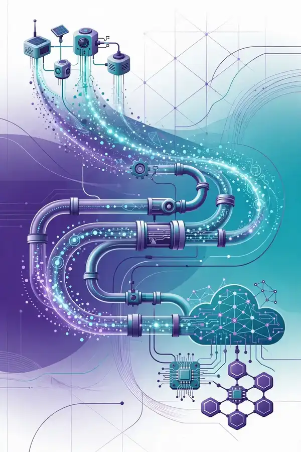
Book 34 of 50 · Free
IoT Data Pipelines Explained
3,062 words · 17 chapters · illustrated
Book 34 of 50 · Free
3,062 words · 17 chapters · illustrated
Book 34 of 50 — AstolixGen Learning Series For researcher and publication students
Sensors produce data; decisions need information. The pipeline between them — ingestion, transport, stream processing, storage, and serving — is where most IoT projects succeed or fail. This book builds the full pipeline mental model: MQTT/CoAP ingestion, stream processors, time-series databases, batch vs stream trade-offs, and exactly-once semantics. You will learn to design, measure, and publish pipeline studies with honest end-to-end numbers.
Learning objectives: - Map the five stages of an IoT data pipeline - Choose ingestion protocols and brokers for scale - Compare stream vs batch processing with measured trade-offs - Select time-series storage (InfluxDB, TimescaleDB) by workload - Reason about delivery semantics: at-most/at-least/exactly-once - Handle late, missing, and out-of-order sensor data - Design a publishable pipeline evaluation
Every IoT data pipeline has five stages. Ingest: devices publish readings (MQTT/CoAP/HTTP) to a broker or gateway. Transport/buffer: a durable log (Kafka, MQTT broker with persistence) absorbs bursts and decouples producers from consumers. Process: stream processors (Flink, Spark Streaming, or simple consumers) clean, aggregate, detect events, and enrich. Store: hot data in time-series DBs for dashboards, cold data in object storage for training. Serve: APIs, dashboards, alerts, and ML training jobs consume the data.
Failures concentrate at the joints: ingest without buffering loses data during outages; processing without idempotency double-counts on replay; storage without retention policy grows forever and bankrupts the project. Draw your pipeline as a diagram before writing any code — then label each arrow with data rate, format, and delivery guarantee. That diagram belongs in every IoT paper.
Example: A 500-sensor farm pipeline: sensors → MQTT (Mosquitto) → Telegraf → InfluxDB (hot, 30-day retention) → nightly export to Parquet on disk (cold) → Grafana dashboards + weekly training job. Each joint labeled: 500 msg/min, JSON, at-least-once.
For your research: The pipeline diagram with rates and guarantees is a required figure in systems papers. Reviewers check that every arrow is justified.
Key takeaway: Ingest → buffer → process → store → serve — label every joint with rate, format, and guarantee.
Ingestion is the narrow waist: everything flows through it. For under ~10k msg/s, a single Mosquitto or EMQX node suffices; beyond that, you need clustered brokers (EMQX, HiveMQ) or a Kafka fronted by MQTT (via Kafka's MQTT proxy or a bridge). Protocol choice at ingest follows Book 31/33: MQTT for pub/sub fan-out, CoAP for UDP-constrained links, HTTP for simplicity.
The key ingestion metrics: throughput (msg/s sustained), fan-in (concurrent publishers), p99 ingest latency, and behavior under backpressure (what happens when consumers lag — drop? buffer? block?). Test backpressure explicitly: kill the consumer for 60 seconds and observe. Systems that silently drop data fail open in dangerous ways.
Example: A campus deployment: 2,000 sensors × 1 msg/10 s = 200 msg/s — trivially handled by one Mosquitto instance at <5% CPU. The same team later added 50 cameras' metadata at 30 msg/s each and hit Mosquitto's single-node ceiling — migrating to EMQX clustered took a weekend because topics were unchanged.
For your research: Ingestion benchmarks (broker X vs Y at N publishers) are clean, reproducible papers — provided you report hardware, message sizes, QoS, and the backpressure policy.
Key takeaway: Size ingestion for 10× your current load; test backpressure; keep topics stable across broker migrations.
Stream processing handles each event as it arrives (milliseconds to seconds of latency): alerting, live dashboards, online control. Batch processing handles bounded datasets on a schedule (minutes to hours): daily reports, model retraining, billing. Micro-batch (Spark Streaming's model) is a middle ground with seconds of latency.
Choose by the decision's timescale: a gas-leak alert cannot wait for the nightly batch; a monthly yield report gains nothing from streaming. Many systems do both from the same log (the "Kappa" idea): the stream serves real-time needs, and replays of the log serve batch needs — one ingestion path, two consumers.
The research-relevant trade-off: streaming systems are harder to make correct (out-of-order data, exactly-once) and their evaluation must include late-data handling. Batch is simpler and reproducible. A paper should justify the choice against the application's latency requirement, stated numerically.
Example: Cold-chain monitoring: stream path — temperature > 8°C for 10 min → SMS alert within 60 s. Batch path — nightly: compute per-truck compliance scores, retrain the spoilage-risk model weekly. Same MQTT topics feed both.
For your research: If you propose a streaming algorithm, evaluate it against a batch baseline on the same data and report the latency/accuracy trade-off. "Streaming" alone is not a contribution.
Key takeaway: Match processing model to decision latency; justify streaming with a numeric latency requirement.
Sensor data is time-series: timestamped, append-only, queried by time range and tag. General databases handle it poorly at scale. InfluxDB (tag-set model, built-in downsampling/retention) excels at high-ingest monitoring. TimescaleDB (PostgreSQL extension, hypertables) excels when you need SQL joins with relational data. Tiering is the cost control: hot tier (SSD, days–weeks) for dashboards, warm tier (compressed, months), cold tier (Parquet on object storage, years) for training and audit.
Design decisions: schema (one measurement per metric vs wide rows — the former scales better), retention policies (drop raw after 30 days, keep 1-min rollups for a year), and downsampling tasks (continuous aggregates). Get retention wrong and storage costs grow unboundedly — the most common IoT project failure after security.
Example: 1,000 sensors × 1 reading/10 s × 50 bytes = 432 MB/day raw. Hot: 14 days raw (6 GB). Warm: 1-min averages for 1 year (105 MB). Cold: Parquet yearly archives. Total manageable; without downsampling, 5-year raw retention would be 788 GB.
For your research: Storage benchmarks (ingest rate, query latency for typical dashboard queries, compression ratio) across InfluxDB/TimescaleDB on identical workloads are useful, citable systems work.
Key takeaway: Use time-series DBs, design retention + downsampling on day one, tier by access pattern.
At-most-once: messages may be lost, never duplicated (MQTT QoS 0). At-least-once: messages never lost, may be duplicated (QoS 1, Kafka default) — consumers must be idempotent (processing a duplicate changes nothing). Exactly-once: each message processed once (QoS 2 per-hop, Kafka transactions + idempotent producer) — expensive and often unnecessary.
The pragmatic rule: use at-least-once everywhere and make consumers idempotent (keyed writes, deduplication on message IDs). Reserve exactly-once for money and safety. Most IoT analytics (averages, counts over windows) tolerate duplicates if you dedupe by (device_id, timestamp) — a 10-line change that removes the need for expensive exactly-once machinery.
Example: A rainfall counter double-counting due to QoS 1 redelivery overstated irrigation by 8%. Fix: consumer keyed on (sensor_id, reading_ts) with "insert if not exists" — duplicates became harmless, no protocol change needed.
For your research: Semantics papers should demonstrate the failure: show duplicate rates under redelivery, quantify the error without dedup, then show the fix. Measured failure + fix is a complete story.
Key takeaway: At-least-once + idempotent consumers beats exactly-once machinery for most IoT analytics.
Real sensor data is messy. Late data arrives after its window closed (network delay). Out-of-order data arrives with earlier timestamps after later ones. Missing data never arrives (dead sensor, lost packets). Your pipeline must define policies: watermarks (how long to wait for late data), allowed lateness, and gap-filling (forward-fill, interpolate, or mark missing — never silently fabricate).
For ML, data quality is a first-class concern: a model trained on silently-interpolated gaps learns fiction. Log data-quality flags alongside readings (was_interpolated, gap_seconds) so training pipelines can exclude or weight suspect data.
Example: A vibration monitor's 2% packet loss created gaps that a naive pipeline forward-filled — the anomaly detector then "detected" the flat lines as anomalies. Fix: propagate a data-quality flag; the detector learned to ignore flagged windows. False alarms dropped 60%.
For your research: Data-quality handling is an under-published topic. A paper characterizing gap patterns in a real deployment and evaluating mitigation strategies fills a genuine gap.
Key takeaway: Define late/out-of-order/missing policies explicitly; propagate quality flags to ML.
Choose a wire format deliberately. JSON is human-readable and debuggable but verbose (bad for LoRa). CBOR/MessagePack are binary JSON — 40–60% smaller, still schemaless. Protobuf/Avro need schemas but give the smallest payloads and safe evolution (additive field changes). Rule: JSON for gateways and debugging, binary for constrained links, schema-based when multiple teams consume the data.
Schema evolution is where projects rot: a firmware update adds a field and breaks the dashboard. Use a schema registry (or at minimum versioned topics like v2/...), enforce backward-compatible changes (only add optional fields), and test old consumers against new producers in CI.
Example: Adding battery_mv to a sensor payload: with Protobuf, old consumers ignore the new field — zero downtime. With ad-hoc CSV, the dashboard parsed the wrong column for a week. The paper's lesson section was titled "use schemas."
For your research: Format comparisons (bytes per message, parse time on MCU, energy) across JSON/CBOR/Protobuf on your hardware are compact, useful measurements.
Key takeaway: Binary + schemas for constrained links; version everything; test evolution in CI.
Monitor the pipeline, not just the sensors. Golden signals: throughput (msg/s per stage — a drop means blockage), lag (consumer offset behind the log — growing lag means under-provisioning), error rate (parse failures, auth failures), duplication rate (are idempotency keys working?), and end-to-end latency (sensor timestamp → dashboard render).
Alert on pipeline health, not just sensor values: "ingest lag > 5 min" pages the engineer before the dashboard goes stale. Keep a dead-letter queue for unparseable messages — every one is a bug report from the field.
Example: A farm dashboard froze every night at 2 AM. Pipeline metrics showed the batch export locking the hot DB — the fix (read replica for exports) was obvious once lag and query-latency were graphed. The postmortem became a conference talk.
For your research: Observability studies — what to monitor, alert thresholds derived from data — are practical contributions that industry tracks value.
Key takeaway: Monitor throughput, lag, errors, duplication, and end-to-end latency; alert on pipeline health.
Push processing to the edge where it pays: filtering (send only interesting events), aggregation (1-min averages instead of 1-s raw), compression (delta encoding), and event detection (thresholds, tiny models). The pipeline then handles orders of magnitude less data, and the cloud bill collapses.
The design question is what the edge may discard: raw data needed for future model training must still be sampled (store 1% raw or event-centered windows). "Filter everything" destroys your future training set — a common regret.
Example: Acoustic pest trap: edge classifier scores every 10 s of audio; only scores > 0.7 upload a 5-s clip; 1% random raw samples upload for retraining. Uplink: 2.4 GB/day → 31 MB/day. Retraining data preserved via sampling.
For your research: Edge-filtering papers must report the preservation metric: what fraction of true events survived filtering (recall at the filter stage), not just the data reduction.
Key takeaway: Filter and aggregate at the edge, but sample raw data for future training; report filter recall.
Each stage is an attack surface. Ingest: TLS, per-device credentials, topic ACLs (Book 31). Transport: encrypt the log, authenticate consumers. Processing: validate and sanitize inputs (a malicious sensor can inject payloads that break parsers — fuzz your parsers). Storage: encrypt at rest, least-privilege DB roles, audit logs. Serve: authenticated APIs, rate limiting.
The pipeline-specific risk is data integrity: an attacker who can inject plausible sensor readings can manipulate decisions (fake "all clear" from a safety sensor). Sign readings at the device (HMAC with a device key) and verify at ingestion — integrity, not just confidentiality.
Example: A building-management pipeline accepted unsigned JSON; a compromised thermostat injected "CO2 normal" during a real ventilation failure. Post-incident: HMAC-signed CBOR at the device, verification at the broker bridge, alerts on signature failures.
For your research: Pipeline security analyses — threat model per stage, measured cost of HMAC/TLS on the device — are strong applied-security contributions.
Key takeaway: Secure every stage; sign sensor data at the source for integrity, not just TLS for confidentiality.
Pipeline costs hide in: ingest (per-message broker/cloud fees), storage (hot tier $/GB-month), processing (always-on stream workers), and egress (dashboards pulling data out of the cloud). Model each: monthly = ingest_msgs × fee + hot_GB × rate + worker_hours × rate + egress_GB × rate. Then attack the biggest term: downsample sooner, filter at edge, cache dashboards, move cold data to cheap object storage.
Example: A 5,000-sensor pipeline cost $1,900/month: 55% hot storage, 25% stream workers, 20% ingest. Cutting hot retention 30→7 days and adding edge aggregation saved $1,100/month with no dashboard change — the cost teardown was the paper's most-read section.
For your research: Cost teardowns of real pipelines are rare and valuable. Anonymize the deployment, show the model, show the optimization — industry citations follow.
Key takeaway: Model cost per stage, attack the biggest term, publish the teardown.
Template:
Write in IEEE format; the architecture diagram is Figure 1; evaluation leads with the end-to-end numbers.
For your research: This is your A1→A4 pipeline again: problem + lit review, method, results, presentation — now for data infrastructure.
Key takeaway: Pain → hypothesis → five-stage design → fault-injected evaluation → artifact = a publishable pipeline paper.
| # | Chapter | Core idea | Research use |
|---|---|---|---|
| 1 | Pipeline model | 5 stages, labeled joints | Architecture figure |
| 2 | Ingestion | Brokers, backpressure | Broker benchmarks |
| 3 | Stream vs batch | Decision-latency rule | Justify with numbers |
| 4 | TS storage | InfluxDB/TimescaleDB, tiers | Storage benchmarks |
| 5 | Semantics | At-least-once + idempotency | Failure demos + fixes |
| 6 | Messy data | Late/missing/out-of-order | Gap-pattern studies |
| 7 | Formats | JSON→CBOR→Protobuf | Format measurements |
| 8 | Observability | Lag, duplication, e2e latency | Monitoring studies |
| 9 | Edge processing | Filter + sample raw | Filter-recall reporting |
| 10 | Security | Per-stage threats, signed data | Threat models + costs |
| 11 | Cost | Per-stage model, teardown | Published cost analyses |
| 12 | Study template | Pain→hypothesis→artifact | A1–A4 mapping |
[1] L. Atzori, A. Iera, and G. Morabito, "The Internet of Things: A survey," Computer Networks, vol. 54, no. 15, pp. 2787–2805, 2010. [2] A. Banks and R. Gupta, "MQTT Version 3.1.1," OASIS Standard, Oct. 2014. [3] W. Shi, J. Cao, Q. Zhang, Y. Li, and L. Xu, "Edge Computing: Vision and Challenges," IEEE Internet of Things Journal, vol. 3, no. 5, pp. 637–646, 2016. [4] M. Satyanarayanan, "The Emergence of Edge Computing," Computer, vol. 50, no. 1, pp. 30–39, 2017. [5] J. Kreps, N. Narkhede, and J. Rao, "Kafka: A distributed messaging system for log processing," in Proc. NetDB Workshop, 2011. [6] T. Akidau et al., "The Dataflow Model: A practical approach to balancing correctness, latency, and cost in massive-scale, unbounded, out-of-order data processing," Proc. VLDB Endowment, vol. 8, no. 12, 2015. [7] S. Wolfert, L. Ge, C. Verdouw, and M. J. Bogaardt, "Big Data in Smart Farming — A review," Agricultural Systems, vol. 153, pp. 69–80, 2017. [8] R. Roman, P. Najera, and J. Lopez, "Securing the Internet of Things," Computer, vol. 44, no. 9, pp. 51–58, 2011. [9] ISO/IEC 20922:2016, "Information technology — MQTT v3.1.1," 2016. [10] H. Kopetz, Real-Time Systems: Design Principles for Distributed Embedded Applications, 2nd ed. Springer, 2011. (book)
End of Book 34. Next: Book 35 — Smart Agriculture with IoT.