Book 29 of 50 · Free

IoT Fundamentals: Devices, Sensors, Networks

24,637 words · 17 chapters · illustrated

IoT Fundamentals: Devices, Sensors, Networks

Book 29 of 50 — AstolixGen Learning Series For researcher and publication students

Book cover — connected IoT devices

About This Book

This book is a deep, practical introduction to the Internet of Things (IoT) for MS and PhD students and early researchers. Many theses today — in agriculture, environment, health, energy, and smart cities — depend on sensor data. Yet most students learn IoT in fragments: a sensor here, a protocol there, a dashboard somewhere else. This book connects the fragments into one coherent picture: how a physical quantity becomes an electrical signal, how that signal becomes a number inside a microcontroller, how the number travels over a network, and how it finally becomes a decision or a published result.

You do not need electronics experience to follow this book. Every concept is explained in plain language first, then tied to real components you can actually buy and to research questions you can actually publish on. The book is deliberately hardware-grounded: it names the parts (ESP32, DHT22, LoRa modules, relays, MQTT brokers), compares them honestly, and shows you how to reason about trade-offs — range versus power, cost versus accuracy, edge versus cloud — the way reviewers and supervisors expect a researcher to reason.

Learning objectives. By the end of this book, you will be able to:

Define IoT precisely and describe its standard architecture layers, from perception to application.
Explain how common sensors (temperature, humidity, motion, gas, light) convert physical quantities into electrical signals.
Select an appropriate sensor for a research experiment using accuracy, cost, and interface criteria.
Describe how actuators (relays, DC motors, servos) are driven from a microcontroller and why power isolation matters.
Compare ESP32, Arduino boards, and Raspberry Pi on processing power, networking, power consumption, and use case.
Evaluate connectivity options (Wi-Fi, Bluetooth/BLE, LoRa/LoRaWAN, Zigbee, cellular) using range, power, and data-rate trade-offs.
Explain MQTT publish/subscribe in depth and contrast it with HTTP and CoAP.
Decide where computation should happen (edge vs cloud) for a given research scenario.
Trace a complete IoT data pipeline from sensor reading to dashboard, including timestamping, buffering, and storage.
Design a complete, budgeted IoT research prototype — parts list, wiring plan, and data plan — suitable as a thesis proposal appendix.

Chapter 1: What Is the Internet of Things?

1.1 A working definition

The Internet of Things (IoT) is the network of physical objects — "things" — that are embedded with sensors, software, and connectivity so they can collect data and exchange it with other systems over the internet. The crucial word is things: not laptops and phones, but thermostats, soil probes, street lamps, water meters, door locks, industrial motors, and livestock tags. What makes them "IoT devices" is that they sense the physical world, communicate digitally, and usually act on it in some way.

A narrower definition used in research papers is helpful because it sets a boundary: an IoT system is a system in which physical-world measurements are digitized at the source, transmitted over a network, and used for monitoring, analysis, or automated control, with human intervention optional. Keep this definition in mind — it distinguishes genuine IoT from a device that merely has Wi-Fi (like a connected toothbrush app, which is really just Bluetooth telemetry).

1.2 A brief history

IoT did not arrive suddenly; it is the convergence of several older threads.

1980s–1990s: embedded systems and machine-to-machine (M2M). Industrial controllers (PLCs), vending machines, and SCADA systems already exchanged data with central servers, usually over wired or dial-up links. This was IoT without the internet ubiquity.
1999: the term "Internet of Things." Kevin Ashton of Procter & Gamble coined the phrase while working on RFID supply-chain tracking — he argued that computers needed their own way to "see" the world through sensors, rather than relying on data typed in by humans.
2000s: RFID and wireless sensor networks. Researchers built "motes" — tiny battery-powered sensor nodes that formed mesh networks. Projects like Great Duck Island (2002, habitat monitoring) showed that low-power wireless sensing worked in the field, but batteries and fragile radios were the pain points.
2008–2014: the smartphone dividend. MEMS sensors (accelerometers, gyroscopes), cheap microcontrollers, and cheap wireless radios became abundant because phones drove their prices down. The Arduino ecosystem made prototyping accessible to non-engineers, and the ESP8266 (released 2014) put Wi-Fi on a board costing a few dollars — arguably the single event that made hobbyist and research IoT practical.
2015–2020: cloud IoT platforms. Major cloud providers offered managed IoT services (device registration, MQTT brokers, time-series storage), which let researchers deploy at scale without building infrastructure.
2020s: edge AI and LPWAN maturity. LoRaWAN networks matured for long-range low-power sensing; tiny machine-learning models ("TinyML") started running directly on microcontrollers; 5G and NB-IoT addressed industrial and wide-area needs.

1.3 Scale — why researchers care

Industry analysts have repeatedly estimated tens of billions of connected IoT devices worldwide, with forecasts in the range of 30 billion+ devices by 2030 (estimates vary by source, so always cite the specific forecast you use). The exact number matters less than the trend: sensing is becoming the cheapest way to obtain ground-truth data about the physical world. For a researcher, this changes the economics of data collection. A decade ago, a year of hourly soil-moisture readings from a farm meant manual visits or expensive data loggers. Today it means a €/$30 node and a spreadsheet of 8,760 timestamped rows. When data collection becomes cheap, the research bottleneck moves from collecting data to asking the right questions about it — which is exactly where you, as a researcher, add value.

1.4 The standard architecture: layers of an IoT system

Nearly every IoT paper and system diagram uses some version of a layered architecture. The four-layer model below is the one most textbooks and papers use; learn it, because it gives you a vocabulary for your methodology chapter.

Layer	What it does	Examples
Perception (device) layer	Senses the physical world and performs physical actions	Temperature sensors, soil probes, cameras, relays, motors
Network (transport) layer	Moves data between devices and the rest of the system	Wi-Fi, LoRa, BLE, Zigbee, cellular, MQTT, CoAP
Processing (middleware/edge-cloud) layer	Stores, cleans, aggregates, and analyzes data; runs rules and models	Gateways, MQTT brokers, time-series databases, cloud functions, ML models
Application layer	Delivers value to users: dashboards, alerts, automation rules, reports	Web dashboards, mobile apps, SMS alerts, automated irrigation schedules

Some models split the processing layer into edge (processing on or near the device) and cloud (processing on remote servers) — Chapter 7 covers that decision in depth. Others add a business layer on top (billing, analytics-as-a-service). For your thesis, the four-layer model is usually sufficient, and drawing your system on it shows the reviewer you understand the full stack.

IoT vs M2M (machine-to-machine): M2M is device-to-device communication, often closed and proprietary. IoT adds internet protocols, interoperability, and data analytics.
IoT vs WSN (wireless sensor networks): A WSN is the networking layer of an IoT system — the nodes and radios. IoT is the full stack from sensor to application.
IoT vs cyber-physical systems (CPS): CPS emphasizes tight feedback loops between computation and physical processes (e.g., an autonomous drone). All CPS are IoT-adjacent, but not all IoT has real-time control.
IoT vs embedded systems: An embedded system is a computer inside a device (a washing-machine controller). It becomes IoT when it connects to a network and participates in a larger data system.

1.6 Why IoT is a research goldmine for students

IoT sits at the intersection of cheap hardware and hard problems: calibration, reliability, power, security, and scale are all unsolved in practice. This means a student with a few hundred dollars of hardware can produce a publishable contribution — a better calibration method for low-cost sensors, an energy-saving transmission schedule, a comparison of two protocols on real hardware. Your advantage over industry is not budget; it is the patience to measure carefully and the obligation to report honestly, including failures. Reviewers value that.

1.7 IoT verticals: where the research lives

IoT is not one market but many, each with its own constraints and publication venues:

Smart agriculture: soil sensing, irrigation control, livestock tracking, greenhouse automation. Constraints: no power, no connectivity, harsh weather, cost per node critical. This is the most accessible vertical for student research — a farm is a willing testbed and the problems are real.
Environmental monitoring: air quality, water quality, noise, flood detection. Constraints: calibration against reference instruments, long unattended durations, public-data credibility. Strong fit for thesis work because the data has civic value.
Smart buildings/cities: occupancy, energy metering, HVAC optimization, street lighting, waste management. Constraints: working around existing infrastructure, stakeholder permissions, privacy.
Industrial IoT (IIoT): predictive maintenance (vibration, temperature of machinery), asset tracking, process control. Constraints: reliability demands, safety certification, legacy equipment integration. Harder for students to access, but case studies with a local factory are gold.
Healthcare/wearables: vital-sign monitoring, fall detection, medication adherence. Constraints: medical accuracy requirements, ethics approval, privacy regulation. High impact, high bar.
Smart home: the most crowded space — thermostats, locks, energy plugs. Fine for learning, weak for novel research unless you address security or energy.

Pick a vertical early. It determines your test site, your reference instruments, and which journals will care about your results.

1.8 Standards and governance (know the names)

IoT's alphabet soup of standards bodies matters when you write related work:

oneM2M: a global partnership developing a common service layer for M2M/IoT — the "write once, run on any network" vision.
W3C Web of Things (WoT): describes devices with machine-readable "Thing Descriptions" so different ecosystems interoperate. If your thesis touches interoperability, cite WoT.
ITU-T: the UN telecom agency's IoT work (notably the Y.4000 series recommendations defining IoT reference models).
IETF: maintains CoAP, 6LoWPAN, and other constrained-device protocols (RFCs you can cite directly).
LoRa Alliance / CSA (Connectivity Standards Alliance, formerly Zigbee Alliance): industry alliances behind LoRaWAN and Matter/Zigbee.

You don't need to master these, but dropping the right standard into your related-work section signals literacy to reviewers.

1.9 Architecture variants: 3-layer vs 5-layer

The four-layer model in §1.4 is the teaching standard, but papers vary:

3-layer (perception / network / application): the simplest; fine for small systems where processing is trivial.
5-layer (perception / transport / processing / application / business): adds an explicit business layer (billing, user management, analytics products) — common in commercial IoT platform papers.

Choose the model that fits your system and say which one you use. A methodology sentence like "We adopt the four-layer IoT architecture (perception, network, processing, application)…" costs nothing and prevents reviewer confusion.

1.10 IoT data: volume, velocity, variety

IoT data has the classic "big data" traits, and naming them helps you design for them:

Volume: a single vibration sensor at 1 kHz produces 86 million samples a day. You cannot store everything raw — aggregation and retention policies (Chapter 8) are mandatory, not optional.
Velocity: readings arrive continuously; your ingestion must keep up in real time. Design for peak rate, not average.
Variety: numeric time series, images, audio, event logs, GPS tracks — your storage and schema must handle mixed types.
Veracity: sensors lie (drift, noise, failures) — data-quality pipelines (Chapter 11) exist because of this trait.
Value: most raw readings are boring; the value is in the exceptions and aggregates. "Send insights, not raw streams" (Chapter 7) is the design response.

A thesis methodology that names these traits for its own data ("our deployment generates ~2.7 M readings; we retain raw for 90 days…") shows the reviewer you understand scale.

1.11 The economics that make IoT research possible

Put numbers on why this book's approach works for students: a research-grade sensing point (ESP32 + digital sensor + enclosure + power) costs roughly $15–40 in parts. A 20-node deployment is $300–800 — within a typical MS thesis budget. The expensive parts of research IoT are not the parts: they're your time (firmware, calibration, field visits) and the reference instruments (borrowed, rented, or accessed via public data). Budget your time the way Chapter 12 budgets parts: 2–4 weeks build, 1–2 weeks bench calibration, deployment, then months of mostly-automated collection while you read literature and write. The hardware works while you sleep — that is the economic miracle of IoT research.

For your research: IoT papers in indexed journals typically contribute in one of these ways: (1) a novel low-cost sensing setup validated against reference instruments; (2) an energy-efficiency improvement with measured battery life; (3) a comparative evaluation of protocols/platforms on real hardware; (4) a dataset collected over weeks/months and released publicly; (5) a deployed system in a real environment (farm, hospital ward, building) with lessons learned. Before you start, pick which lane your work will be in — it shapes everything from your parts list to your literature review.

Key takeaways:

IoT = physical things that sense, communicate, and act, connected through internet protocols.
The field grew from M2M/SCADA through RFID, wireless sensor networks, cheap Wi-Fi microcontrollers, and cloud platforms.
Learn the four-layer architecture (perception → network → processing → application); it structures every IoT paper and thesis.
Cheap hardware moved the research bottleneck from data collection to good questions — your comparative advantage.

Chapter 2: Sensors — The Eyes and Ears

Common sensor types

2.1 What a sensor actually does

A sensor converts a physical quantity (temperature, pressure, light, motion) into an electrical signal (usually a voltage or current) that electronics can process. That signal is then converted to a digital number by an analog-to-digital converter (ADC), and the microcontroller turns the number into a measurement using a calibration formula.

This chain — physical → electrical → digital → calibrated value — is the foundation of every IoT measurement. Whenever a reading looks wrong, walk the chain backwards: Is the physical stimulus reaching the sensor (blocked vent? sensor in sunlight?)? Is the electrical signal sane (check with a multimeter)? Is the digital conversion configured correctly (ADC resolution, reference voltage)? Is the calibration formula right? Roughly 80% of "broken sensor" problems are in the physical setup, not the chip.

Two sensor families matter most:

Analog sensors output a continuously varying voltage. Example: a TMP36 temperature sensor outputs 750 mV at 25 °C, changing by 10 mV per °C. You read it with the ADC and compute temperature from the voltage. Analog sensors are cheap but sensitive to electrical noise and supply-voltage drift.
Digital sensors contain their own ADC and signal conditioning, and report numbers over a digital interface (I²C, SPI, UART, or a one-wire protocol). Example: the DHT22 reports temperature and humidity as digital values. They cost slightly more but are far easier to use reliably, and most research prototypes should prefer them.

2.2 How the common sensors work

Temperature sensors

Thermistors (NTC/PTC): resistors whose resistance changes strongly with temperature. NTC thermistors drop in resistance as they heat up. They are cheap and sensitive, but the resistance–temperature curve is nonlinear, so you need a lookup table or the Steinhart–Hart equation to convert. Common in 3D printers and HVAC.
RTDs (e.g., PT100): platinum resistors with a nearly linear, very stable response. The reference standard for accurate temperature measurement (industrial, laboratory). More expensive and need careful analog circuitry.
Thermocouples: two joined dissimilar metals produce a small voltage proportional to the temperature difference (Seebeck effect). They measure very high temperatures (furnaces, engines) but need a "cold-junction compensation" circuit and an amplifier.
Digital temperature ICs (DS18B20, DHT22, SHT-series): a temperature-sensing element plus ADC and digital interface in one package. The DS18B20 (±0.5 °C accuracy, one-wire bus, waterproof probe versions exist) is the workhorse for research fieldwork because you can put many on one wire and dunk them in water or soil.

Humidity sensors

Most humidity sensors are capacitive: a polymer film absorbs water vapor, changing its capacitance, which an on-chip circuit converts to relative humidity (RH). The DHT11 (cheap, ±5% RH, slow) and DHT22/AM2302 (±2–5% RH, wider range) are the common hobbyist parts; the SHT31/SHT35 family offers better accuracy (±2% RH) and an I²C interface. Key research fact: humidity sensors drift over time and are contaminated by dust, condensation, and some gases — budget for periodic recalibration against a reference.

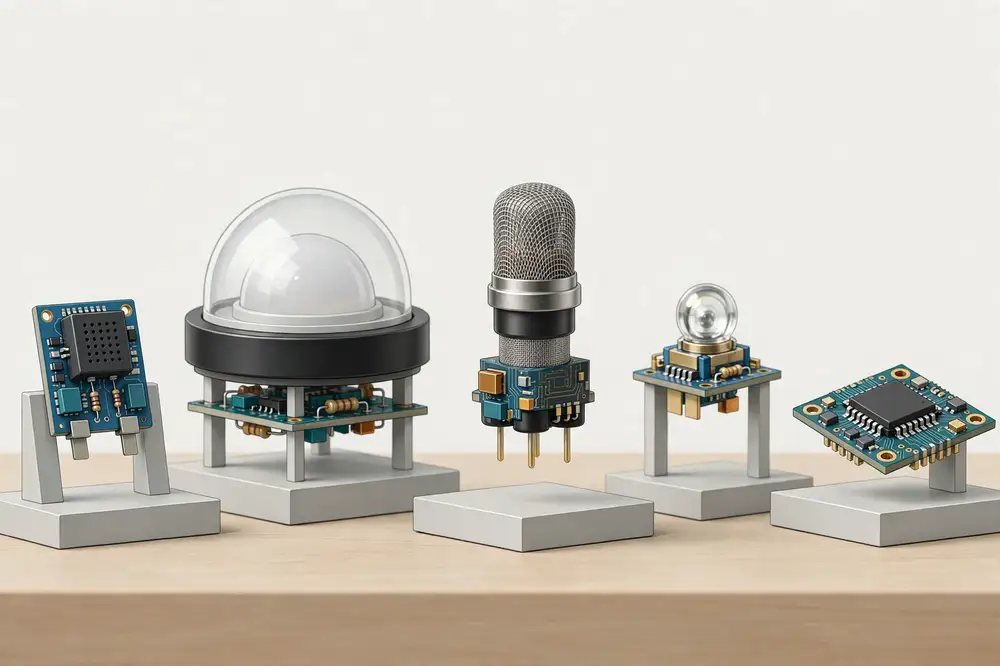
Motion and presence sensors

PIR (passive infrared): detects changes in infrared radiation from warm bodies moving across its field of view. The classic white-domed sensor on security lights. Cheap and very low power, but it only detects movement, not presence — a person sitting still eventually becomes invisible to it. Range is typically several meters.
Ultrasonic (HC-SR04): emits sound pulses above human hearing and times the echo to measure distance (like a bat). Good for liquid-level measurement and parking sensors; accuracy suffers with soft or angled surfaces.
Microwave/Radar: emits radio waves and detects Doppler shift from movement. Sees through non-metallic walls — useful for occupancy detection but raises privacy considerations in human studies.
Accelerometers (MPU6050, ADXL345): MEMS chips that measure acceleration along axes, used for vibration monitoring, fall detection, and tilt sensing. Most modern ones report digitally over I²C.

Gas and air-quality sensors

MQ-series (MQ-2, MQ-135, etc.): metal-oxide semiconductor sensors whose resistance changes in the presence of target gases (smoke, LPG, CO, general "air quality"). Very cheap and widely used in student projects — but they are not selective (MQ-135 responds to many gases), need a burn-in/warm-up period (the heater must stabilize, often 24–48 hours for stable baseline, minutes for rough readings), and give only relative readings unless carefully calibrated against a reference instrument. A common research contribution: characterizing and calibrating an MQ sensor against a reference for a specific environment.
NDIR CO₂ sensors (MH-Z19, SCD30): use nondispersive infrared absorption — CO₂ absorbs specific IR wavelengths, so measuring absorption gives a selective CO₂ reading. Far more trustworthy than MQ-series for CO₂; the SCD30 also reports temperature and humidity.
Particulate matter (PMS5003, SDS011): laser-scattering sensors that count particles to estimate PM2.5/PM10. Hugely popular for low-cost air-quality networks; research consistently shows they need humidity correction and collocation calibration against reference monitors.

Light sensors

LDR (photoresistor): resistance falls as light increases. Extremely cheap, very nonlinear, slow — fine for "is it day or night" decisions, useless for precise lux measurement.
Photodiodes/phototransistors: faster, more linear; used with an amplifier circuit.
Digital ambient-light sensors (BH1750, TSL2561): report illuminance in lux over I²C with good linearity. Use these when your research needs real numbers.

2.3 Sensor selection: the researcher's decision table

Criterion	What to ask	Why it matters for research
Accuracy & precision	What is the datasheet accuracy? What did independent tests find?	Defines your error bars; reviewers will challenge uncalibrated claims
Range	Does it cover your expected conditions (e.g., −10 to 50 °C)?	Out-of-range readings are silently wrong
Interface	Analog, I²C, SPI, UART, one-wire?	Determines wiring complexity and how many sensors share a microcontroller
Power	Active current, sleep current, warm-up time	Battery-life math (Chapter 10) depends on this
Response time	Seconds or minutes to react?	Matters for control loops and event detection
Stability/drift	How fast does calibration degrade?	Sets your recalibration schedule
Cost	Unit price × number of nodes	Multi-node deployments multiply every dollar
Form factor	Waterproof? Probe-style?	Field deployment reality check

Golden rule: the datasheet is a starting claim, not a fact. For any measurement your paper depends on, collocate your sensor with a reference instrument (a calibrated thermometer, a borrowed data logger, a government air-quality station's public data) for at least a few days, and report the comparison. That single paragraph — "we validated against X, mean absolute error was Y" — is what separates a student demo from a research contribution.

2.4 A data-flow walkthrough: reading a DHT22

Wire it: DHT22 has power (3.3–5 V), ground, and a single data pin connected to a microcontroller GPIO (with a pull-up resistor on many boards this is built into the module).
Request: the microcontroller pulls the data line low for ~1 ms, then releases it — this "wakes" the sensor.
Respond: the DHT22 sends 40 bits: 16 bits humidity, 16 bits temperature, 8 bits checksum.
Validate: the microcontroller checks the checksum; if it fails, the reading is discarded (never log failed checksums as data).
Convert: divide the raw integers by 10 → e.g., 456 → 45.6% RH, 231 → 23.1 °C.
Timestamp and store: attach the reading time (from an RTC or NTP) before sending or logging.

Note the failure modes a researcher must handle: the DHT22 cannot be read more often than about once every 2 seconds; reading faster returns stale or failed data. Its humidity element is slow to respond to rapid changes. Document these limits in your methodology — they bound what your data can claim.

2.5 Deep dive: ADC resolution and quantization

When an analog sensor meets a microcontroller, the ADC decides how finely the voltage is sliced. An n-bit ADC divides its reference voltage into 2ⁿ steps:

ADC resolution	Steps	Step size (3.3 V ref)	Typical found in
10-bit	1,024	3.22 mV	Arduino Uno
12-bit	4,096	0.81 mV	ESP32, most ARM MCUs

For a TMP36 (10 mV/°C), a 12-bit ADC resolves ~0.08 °C per step — plenty. But resolution is not accuracy: electrical noise, reference-voltage drift, and the ESP32's known ADC nonlinearity mean the usable accuracy is worse than the step size suggests. Practical rules: average multiple readings (oversampling + averaging 16 samples buys ~2 extra bits of effective resolution and kills random noise), keep analog traces short and away from the Wi-Fi antenna, add a small capacitor at the ADC input to shunt high-frequency noise, and calibrate the ADC against known voltages at least at two points. If your paper's conclusions rest on analog readings, describe this signal chain — reviewers in instrumentation venues expect it.

2.6 Deep dive: digital interfaces — I²C, SPI, UART, 1-wire

Digital sensors speak one of four languages; choosing among them is a wiring and scalability decision:

I²C (Inter-Integrated Circuit): two wires (SDA data, SCL clock) shared by many devices, each with a 7-bit address. Strengths: only 2 pins for dozens of sensors; weaknesses: short distances (centimeters to ~1 m reliably), address collisions (two identical sensors may share an address — check for address-select jumpers or use an I²C multiplexer). The default choice for on-board sensor clusters (SHT31 + BH1750 + pressure sensor on one bus).
SPI (Serial Peripheral Interface): four wires (MOSI, MISO, SCK, plus one chip-select per device). Faster than I²C, full-duplex, no address collisions — but each device costs a chip-select pin. Best for high-speed devices (SD cards, displays, fast ADCs).
UART (serial): two wires (TX/RX), point-to-point, the simplest to debug (you can watch it with a USB-serial adapter). Common for "smart" modules: GPS, PMS5003, MH-Z19, LoRa modules. Downside: one UART per device (most MCUs have 2–3).
1-wire (e.g., DS18B20): one data wire (+ power/ground) for many devices, each with a unique 64-bit factory ID. Brilliant for temperature probes distributed over meters of cable (soil profiles, building risers). Slower, and parasitic-power mode is finicky — power the probes properly in research deployments.

Pull-up resistors (typically 4.7 kΩ on I²C SDA/SCL and 1-wire data) are the #1 wiring gotcha: without them the bus floats and nothing works; many sensor modules include them, but stacking three modules can put pull-ups in parallel and overload the bus. When a sensor "isn't detected," check pull-ups and addresses with an I²C scanner sketch before anything else.

2.7 Signal conditioning and sensor placement

Between the sensing element and the ADC often sits signal conditioning: amplification (tiny thermocouple voltages need ×100+ gain), filtering (RC low-pass to remove noise above your sampling rate), and protection (series resistors, clamping diodes against overvoltage). Digital modules hide this from you; analog designs expose it — another reason research prototypes favor digital sensors.

Placement is a measurement decision, not an afterthought: a temperature sensor in direct sun reads 10–15 °C high (use a radiation shield — a ventilated white enclosure); a humidity sensor near a heat source reads artificially low; a soil probe at the surface tracks evaporation, not root-zone moisture (bury at root depth, typically 15–30 cm for crops); a PM sensor next to a kitchen exhaust measures the kitchen, not the neighborhood. Photograph every placement and record heights, depths, and orientations — this metadata belongs in your thesis appendix and in the released dataset.

For your research: Pick one sensor your thesis will depend on. Find three independent sources (datasheet, a comparison article, a published paper that used it) and record: stated accuracy, measured accuracy in practice, known drift/failure modes, and calibration approach. This one-page "sensor dossier" becomes the measurement subsection of your methodology chapter and preempts the reviewer's hardest questions.

Key takeaways:

Sensors convert physical → electrical → digital → calibrated value; debug failures by walking that chain backwards.
Prefer digital sensors (I²C/one-wire) over analog for research prototypes — they are more reliable and easier to validate.
MQ-series gas sensors are cheap but non-selective and need burn-in; NDIR and laser-scattering sensors are the trustworthy options for CO₂ and PM.
Always validate against a reference instrument and report the error — that is what makes sensor work publishable.

Chapter 3: Actuators — Making Things Move

3.1 Sensing is only half the story

An actuator converts an electrical signal back into physical action: switching a pump on, opening a valve, turning a motor, sounding an alarm. IoT systems that only sense are monitoring systems; systems that also act are control systems. Most impactful research deployments — automated irrigation, smart incubators, ventilation control — are control systems, and control is where the interesting research problems live (stability, timing, safety, energy trade-offs).

The golden rule of actuation: a microcontroller's GPIO pins are signal sources, not power sources. A typical GPIO pin can safely supply on the order of 10–20 mA at 3.3 V — enough to light an LED, nowhere near enough to run a motor or a mains-powered pump. Every actuator circuit is therefore a two-part design: the microcontroller sends a control signal, and a separate power stage (relay, transistor, motor driver) switches the actual load current from its own power supply. Beginners who wire a motor directly to a GPIO pin destroy boards; researchers who understand the signal/power split design reliable systems.

3.2 Relays: switching the big stuff safely

A relay is an electrically operated switch: a small current through its coil (or, in a relay module, a small signal to its driver circuit) magnetically closes contacts that can switch a much larger load — including mains AC (230 V) appliances like pumps, heaters, and lamps.

Electromechanical relay modules (the common blue "sugar-cube" boards) are cheap, handle AC and DC, and provide physical isolation between the control side and the load side. Downsides: mechanical wear (rated for ~100,000 operations), slow (tens of milliseconds), and they click audibly.
Solid-state relays (SSRs) switch with semiconductors: silent, fast, no wear, but they generate heat at high currents, have small leakage current, and cost more.

Safety — non-negotiable. Mains voltage can kill. Research prototypes switching AC must: use a proper relay module rated above the load current, keep AC wiring physically separated and enclosed, add a fuse, never leave mains prototypes running unattended, and follow your institution's electrical safety rules. If your experiment only needs low-voltage DC (a 12 V pump, a 5 V fan), prefer that — it removes the entire mains-safety problem. State your safety measures in the thesis; ethics/safety reviewers look for them.

3.3 Motors: three kinds you will meet

Motor type	How it works	Control	Typical IoT use
DC motor	Current through coils in a magnetic field spins the shaft; reverse polarity reverses direction	Speed via PWM (pulse-width modulation), direction via an H-bridge driver (e.g., L298N, TB6612FNG)	Pumps, fans, conveyors, simple robots
Servo motor	DC motor + gearbox + position feedback, sealed in one case; moves to a commanded angle	PWM signal where pulse width encodes angle (typically 1–2 ms pulses → 0–180°)	Valve positions, camera pan/tilt, door locks, robot joints
Stepper motor	Moves in discrete steps (commonly 200 steps/revolution) by energizing coils in sequence	Step/direction pulses from a driver (e.g., A4988, DRV8825)	Precise positioning: 3D printers, CNC, automated sampling arms

PWM, the control technique behind DC motor speed and servos, deserves a clear explanation: instead of lowering the voltage (wasteful and weak), the microcontroller switches the full voltage on and off rapidly — hundreds to thousands of times per second. The duty cycle (percentage of time ON) sets the average power: 50% duty cycle ≈ half speed. The motor's inertia smooths the pulses into continuous motion. This is efficient and precise, and it is implemented in hardware on most microcontrollers.

3.4 A data-flow walkthrough: automated irrigation node

Here is how sensing and actuation combine in a classic research prototype — a soil-moisture-triggered irrigation node:

Sense: a capacitive soil-moisture probe (analog output) is read by the ESP32's ADC every 10 minutes. Capacitive probes are preferred over resistive ones because resistive probes corrode in soil within weeks.
Decide: the firmware compares the reading against a threshold (with hysteresis — e.g., turn pump ON below 30% moisture, OFF above 45% — so the pump doesn't chatter on and off at the boundary).
Actuate: the GPIO drives a relay module, which switches a 12 V DC water pump powered by a separate supply. An optoisolated relay module keeps the pump's electrical noise away from the microcontroller.
Report: each state change (pump ON/OFF, with timestamp and moisture value) is published over MQTT so the dashboard shows irrigation events.
Failsafe: a maximum run-time timer (e.g., 5 minutes) forces the pump off even if the sensor fails — because a stuck ON pump floods the field and ruins the experiment. Every actuator in a research deployment needs a failsafe; reviewers ask about them.

3.5 Actuator pitfalls that ruin experiments

Power supply sag: motors and pumps draw large startup (inrush) currents that can brown-out the microcontroller, causing mysterious resets exactly when the pump starts. Fix: separate supplies (or a beefy shared one), thick wires, and capacitors near the motor driver.
Back-EMF: when a motor or relay coil switches off, its magnetic field collapses and generates a voltage spike that can damage electronics. Relay modules include protection; when driving raw coils or motors, use flyback diodes / proper driver ICs.
No feedback: open-loop control ("run pump for 60 seconds") assumes the world cooperates. Closed-loop control ("run until moisture reaches 45%") verifies the result. Research systems should be closed-loop wherever feasible, and should log both the command and the observed outcome.
Mechanical wear: relays, pumps, and valves have finite lives; log actuation counts so you can report duty statistics and replace parts before they fail mid-experiment.

3.6 Deep dive: switching loads with transistors

Relays are not the only power stage. For DC loads, a MOSFET (transistor) switch is cheaper, silent, faster, and longer-lived than a relay:

Low-side switching is the standard pattern: the load's positive terminal connects to the supply, its negative terminal connects to the MOSFET's drain, the MOSFET's source goes to ground, and the GPIO drives the gate. When the GPIO goes high, the MOSFET conducts and current flows through the load.
Use logic-level N-channel MOSFETs (e.g., IRLZ44N type) that fully turn on at 3.3–5 V gate voltage — ordinary power MOSFETs need 10 V and will half-conduct (and overheat) on a GPIO signal.
Add a gate resistor (~100 Ω) to limit inrush current into the gate capacitance, and a pull-down resistor (~10 kΩ) so the MOSFET stays off while the MCU boots (GPIOs float during boot — without the pull-down, motors can twitch on at power-up).
For high-side switching or reversing DC motors, an H-bridge (four switches in an "H" arrangement, packaged in driver ICs like the TB6612FNG) lets current flow either direction through the motor — direction control plus PWM speed in one chip, with built-in flyback protection.

Rule of thumb: MOSFET for DC loads under ~10 A where silence and speed matter; relay where you need AC switching or galvanic isolation; H-bridge driver IC for bidirectional motors.

3.7 Deep dive: servo timing and PWM details

Servo control is a precise timing protocol disguised as simplicity: every ~20 ms the MCU sends a pulse; a 1.0 ms pulse commands 0°, 1.5 ms commands 90°, 2.0 ms commands 180° (conventions vary slightly by manufacturer — verify yours). The servo's internal circuitry measures the pulse width and drives its motor to the matching angle, holding position against load. Key facts for reliable use:

Power: even "micro" servos draw 500+ mA when moving against load and spike higher at stall. Power servos from a separate 5–6 V supply capable of several amps, never from the MCU's regulator — brown-out resets during servo moves are a classic beginner failure.
Jitter: software-generated PWM (bit-banging) jitters under interrupt load; use the MCU's hardware PWM/timer peripherals (ESP32's LEDC/MCPWM, Arduino's Servo library which uses hardware timers) for rock-steady positioning.
Range limits: commanding beyond a servo's mechanical range strains gears; calibrate min/max pulse widths for your specific servo and clamp commands in software.
Continuous-rotation servos trade position control for velocity control (1.5 ms = stop, wider/narrower = spin) — useful for wheels, useless for valves.

3.8 Sizing actuators: torque, current, and duty

Three numbers size every actuator choice:

Torque/force: the valve's required torque, the pump's head pressure, the robot arm's load — measure or estimate the real mechanical demand, then choose an actuator rated at 2× that (the engineering margin covers friction, aging, and your estimation error).
Current: stall current (the maximum the actuator draws when blocked) sizes the power supply and driver — not the running current. A "12 V, 1 A" motor may draw 5 A at stall; size for stall.
Duty cycle: a pump rated for intermittent use will overheat in continuous service. Check the datasheet's duty rating against your control law's expected ON-time.

Document all three in your methodology with the 2× margin stated explicitly — it shows the reviewer you engineered rather than guessed.

3.9 Pumps, valves, and the fluid-control toolkit

Most student control projects move fluids (irrigation, dosing, cooling). The standard parts:

Solenoid valves: electrically opened/closed valves for water/air lines. They come in normally-closed (safe default — power loss stops flow; use these) and normally-open variants, and need a minimum pressure differential on some models — check the specs against your gravity-fed vs pumped setup. Drive via relay or MOSFET like any DC load; add a flyback diode.
Peristaltic pumps: squeeze a tube to move liquid — the fluid never touches the pump mechanism, so they're ideal for dosing fertilizers or chemicals precisely and hygienically. Slow but accurate; great for research dosing rigs.
Diaphragm/submersible pumps: for moving larger volumes (irrigation, drainage). Size by head (vertical lift) and flow rate at that head — a pump rated 5 L/min at zero head may deliver 1 L/min lifting 2 meters.
Water hammer: suddenly closing a valve in a long pipe spikes pressure and can burst fittings. In larger rigs, close valves slowly (PWM ramp on a proportional valve) or add an arrestor. Even at student scale, mount plumbing securely.

Leak discipline: every fluid connection is a future leak. Use proper barbed fittings with hose clamps (not press-fit hope), put a drip tray with a water-leak sensor under indoor rigs, and for unattended operation add a flow meter or leak detector wired as an interlock — if flow occurs when no valve is commanded open, shut everything down and alert. A flooded lab is a memorable but unpublishable result.

For your research: If your thesis involves actuation, your methodology must describe: what is actuated, the control law (thresholds, hysteresis, timing), the failsafes, and the power architecture (separate supplies, driver ratings). "The pump turns on when soil is dry" is a demo description; "the pump activates when the 10-minute median moisture falls below 30% RH-equivalent, deactivates at 45%, with a 5-minute hardware watchdog and logged actuation events" is a research description.

Key takeaways:

GPIO pins carry signals, not power: always use a relay/transistor/driver stage between the microcontroller and any real load.
Relays switch big loads (including mains — with strict safety discipline); DC motors give speed, servos give angle, steppers give precise steps; PWM is the universal control language.
Every actuator needs a failsafe and logged feedback: command + observed outcome, not just command.
Closed-loop control (act, then verify with a sensor) is what makes an IoT deployment a research system rather than a demo.

End of chunk 1 of 4 — continues with Chapters 4–6.

Chapter 4: Microcontrollers and Single-Board Computers

4.1 The brain of the node

Every IoT device needs a "brain" that reads sensors, makes decisions, and talks to the network. Two families of brains dominate IoT, and confusing them is the most common beginner mistake:

A microcontroller (MCU) is a single chip containing a processor, memory (RAM and flash), and peripherals (ADC, timers, GPIO, radios) — everything needed to run one program, forever, on milliwatts of power. It has no operating system; your program runs directly on the hardware ("bare metal" or with a tiny real-time OS). Examples: ESP32, Arduino boards (ATmega328P-based Uno), STM32.
A single-board computer (SBC) is a complete computer on one board: a much faster processor, hundreds of MBs to GBs of RAM, and a full operating system (usually Linux). Examples: Raspberry Pi, Orange Pi, BeagleBone.

The rule of thumb: MCUs sense and act at the edge; SBCs compute, aggregate, and serve. An MCU wakes up, reads a sensor, sends the data, and sleeps — for months on a battery. An SBC runs a database, hosts a dashboard, or processes camera images — but needs continuous watts of power. Research prototypes often use both: MCU nodes in the field, an SBC as a local gateway or edge server.

4.2 The big three, compared honestly

Feature	ESP32 (e.g., ESP32-DevKitC)	Arduino Uno (ATmega328P)	Raspberry Pi (e.g., Pi 4 / Pi 5)
Class	Microcontroller with built-in Wi-Fi + Bluetooth	Microcontroller, no native wireless	Single-board computer, full Linux
Processor	Dual-core 32-bit, up to 240 MHz	Single-core 8-bit, 16 MHz	Quad-core 64-bit ARM, 1.5–2.4 GHz
Memory	~520 KB RAM, 4 MB flash (typical module)	2 KB RAM, 32 KB flash	2–8 GB RAM, microSD storage
Wireless	Wi-Fi + Bluetooth/BLE on-chip	None (needs add-on shields)	Wi-Fi, Bluetooth, Ethernet, USB
Power	~100–200 mA active; deep sleep ~10 µA	~50 mA active; sleep in the mA range without mods	2–5 W+ continuous (no true deep sleep)
Analog inputs	ADC on many pins (12-bit, nonlinear at extremes — calibrate)	6 analog inputs (10-bit ADC)	None natively (needs external ADC)
Programming	Arduino IDE, MicroPython, ESP-IDF	Arduino IDE (C/C++)	Python, any Linux language
Typical price	A few USD	~USD 20+ (genuine); clones cheaper	USD 35+ (board only)
Best for	Battery/Wi-Fi sensor nodes, the default research choice	Teaching, simple wired prototypes, huge tutorial base	Gateways, image processing, dashboards, edge ML

A few honest caveats researchers should know:

The ESP32's ADC is nonlinear near the top and bottom of its range, and its Wi-Fi radio draws large current spikes. Both are manageable (calibrate the ADC; use adequate power supply decoupling), but papers that treat ESP32 ADC readings as precision measurements without calibration get challenged.
The Arduino Uno is electrically 5 V while most modern sensors are 3.3 V — level shifting matters, and its lack of wireless makes it a poor fit for IoT specifically (though fine for wired lab instruments).
The Raspberry Pi is a real computer: it corrupts its SD card if power is yanked mid-write, it needs orderly shutdowns, and it cannot sleep like an MCU. For field deployments, budget for a UPS or use read-only filesystems. Its strength is software: you can run Python, Node-RED, InfluxDB, and a web dashboard on one $50 board.

Other notable MCUs: the ESP8266 (older, cheaper, single-core, Wi-Fi only — still fine for simple nodes), STM32 family (excellent peripherals and low power, steeper learning curve), RP2040 (Raspberry Pi's own MCU, cheap and capable, Wi-Fi only on the Pico W variant), and nRF52 series (the BLE/low-power champion for battery devices).

4.3 How firmware works: the loop

MCU programs follow a simple eternal pattern:

Setup (runs once): configure pins, start the Wi-Fi connection, initialize sensors, sync the clock.
Loop (runs forever): read sensors → process → transmit → sleep → repeat.

For battery nodes, step "sleep" is where the magic happens (Chapter 10): an ESP32 in deep sleep draws roughly 10 µA — effectively off — wakes on a timer, does 2 seconds of work, and sleeps again. A node that wakes for 2 seconds every 10 minutes is awake 0.3% of the time, which is why years of battery life are possible.

Interrupts let the MCU react to events without polling: a PIR motion sensor can wake a sleeping ESP32 instantly via a GPIO interrupt. Timers schedule periodic work. Understanding sleep + interrupts + timers is 90% of embedded firmware for IoT research.

4.4 Choosing the brain: a decision walkthrough

Ask these questions in order:

Does it need Wi-Fi? → ESP32 is the default. No wireless need and simple I/O? → Arduino-class is fine.
Does it run Linux software (database, web server, camera/OpenCV, ML inference)? → Raspberry Pi.
Battery for months? → MCU with deep sleep (ESP32, nRF52). A Pi cannot do this.
How many sensors, and which interfaces? Count I²C/SPI/UART/analog needs against the board's pins.
Operating voltage? 3.3 V sensors pair naturally with ESP32; 5 V legacy sensors pair with Uno (with level shifting either way where mixed).

Document this decision in your thesis ("we selected the ESP32 because…") — it shows engineering judgment, and "why this board" is a standard reviewer question.

4.5 Deep dive: the ESP32 family and Arduino ecosystem variants

"ESP32" is a family, not one chip — knowing the variants prevents buying the wrong board:

ESP32 (classic): dual-core, Wi-Fi + Bluetooth/BLE. The default; the largest tutorial and library base.
ESP32-S3: adds native USB, vector instructions for ML acceleration, and more GPIO — the current best pick for TinyML and camera (ESP32-S3-EYE) projects.
ESP32-C3: single-core RISC-V, Wi-Fi + BLE 5, cheaper and lower power — excellent for simple sensor nodes.
ESP32-C6: adds 802.15.4 (Zigbee/Thread) support — the future-proof choice for Matter/Thread experiments.

Similarly, "Arduino" spans the Uno (teaching classic), Nano (compact, breadboard-friendly), Mega (many pins for complex wired rigs), and modern 32-bit boards like the Nano ESP32 and Portenta (industrial-grade). For IoT research specifically, the 8-bit AVR boards are legacy — fine for teaching, but any wireless project should be on ESP32-class hardware.

Clones vs genuine: cheap clone boards work, but quality varies — voltage regulators that brown out under Wi-Fi load are the classic clone defect. For field deployments, buy from reputable vendors and test every board under full radio load before deployment. A $3 saving is not worth a long round trip to replace a dead node.

4.6 Deep dive: FreeRTOS and multitasking on the ESP32

Unlike Arduino's single loop, the ESP32 runs FreeRTOS, a real-time operating system that lets your firmware do several things "at once" via tasks:

A sensor-reading task (every 5 min), a communications task (MQTT handling), and a watchdog task can run concurrently, each with its own priority and stack.
Queues pass data safely between tasks (sensor task → queue → MQTT task); mutexes/semaphores protect shared resources (don't let two tasks write to the I²C bus simultaneously).
The Arduino-on-ESP32 framework hides FreeRTOS by default (your loop() is just a task), but knowing it exists lets you graduate to non-blocking designs: no more delay() freezing everything — use task delays and timers.

For research firmware, the practical payoff is reliability: a dedicated watchdog task that reboots the board if the comms task hangs for 5 minutes turns mysterious field failures into brief, self-healing hiccups. Log reboot causes (the ESP32 records the reset reason) — a node that reboots nightly at 3 AM is telling you something.

4.7 Raspberry Pi in IoT: roles and hardening

The Pi's IoT roles, from simplest to most ambitious:

MQTT broker + database host (Mosquitto + InfluxDB) for a local sensor network.
Protocol gateway — e.g., BLE sensors → Pi → MQTT/Wi-Fi uplink; LoRaWAN gateway (with a concentrator HAT).
Edge analytics — Node-RED flows, Python anomaly detection, image classification with a camera module.
Field server — serving the Grafana dashboard on a local network with no internet.

Hardening for field use: use an industrial-grade SD card (or better, boot from SSD/USB), mount the filesystem read-only with logs in RAM where possible, add a hardware watchdog (or the Pi's built-in one), power through a UPS, and enable automatic security updates. Document your hardening steps — "the gateway ran 6 months unattended" is a result worth reporting.

4.8 ESP32 pin gotchas every researcher should know

The ESP32 is generous with pins but several have quirks that cause hours of debugging:

Strapping pins (GPIO 0, 2, 5, 12, 15): their state at boot selects boot mode. Holding GPIO 0 low at reset enters download mode (that's how flashing works); accidentally pulling a strapping pin the wrong way with your sensor circuit causes mysterious boot failures. Prefer non-strapping pins for sensors when possible.
ADC2 vs Wi-Fi: on the classic ESP32, the ADC2 peripheral cannot be used while Wi-Fi is active (they share hardware). Use ADC1 pins (GPIO 32–39) for analog sensors on Wi-Fi nodes — this single fact resolves a huge fraction of "my analog readings freeze when Wi-Fi connects" forum posts.
GPIO 34–39 are input-only (no pull-up/pull-down, no output) — fine for sensor inputs, useless for driving relays.
Boot messages: the ESP32 prints boot logs on its UART at 115200 baud — invaluable for debugging; keep a USB-serial connection available on at least one field node.

None of this is in the quick-start tutorials; all of it is in the official Technical Reference Manual [1]. When something "should work but doesn't," the TRM is the authority — learning to read it is a research skill.

4.9 Development environments

Arduino IDE / PlatformIO: the standard path for ESP32 and Arduino. PlatformIO (a VS Code extension) adds proper library management and is what most research labs standardize on.
MicroPython: Python on microcontrollers — faster to write, slower to run, larger memory footprint. Good for prototyping logic; C/C++ wins for tight timing and deep sleep.
ESP-IDF: Espressif's official framework — full control, steeper learning curve, the choice when you need FreeRTOS features or production-grade firmware.
Raspberry Pi OS + Python: standard Linux development; Node-RED gives a visual flow-based option for gateway logic.

For your research: Standardize your lab on one MCU family (ESP32 is the sensible default in 2026) and one toolchain (PlatformIO). Every hour spent fighting a new board's quirks is an hour not spent on your research question. Buy two of every critical part — when a node fails in the field at 9 PM, the spare on your desk is the difference between a lost week and a lost evening.

Key takeaways:

MCUs (ESP32, Arduino) run one program on milliwatts and sleep deeply; SBCs (Raspberry Pi) run Linux on watts and cannot truly sleep.
ESP32 is the default research choice for wireless sensor nodes; Raspberry Pi is the default for gateways, dashboards, and image/ML workloads.
Firmware = setup once + loop forever; deep sleep + interrupts + timers are the core techniques.
Justify your board choice in writing — reviewers ask "why this hardware."

Chapter 5: Connectivity — Wi-Fi, Bluetooth/BLE, LoRa, Cellular, Zigbee

Wireless range comparison

5.1 The iron triangle: range, power, data rate

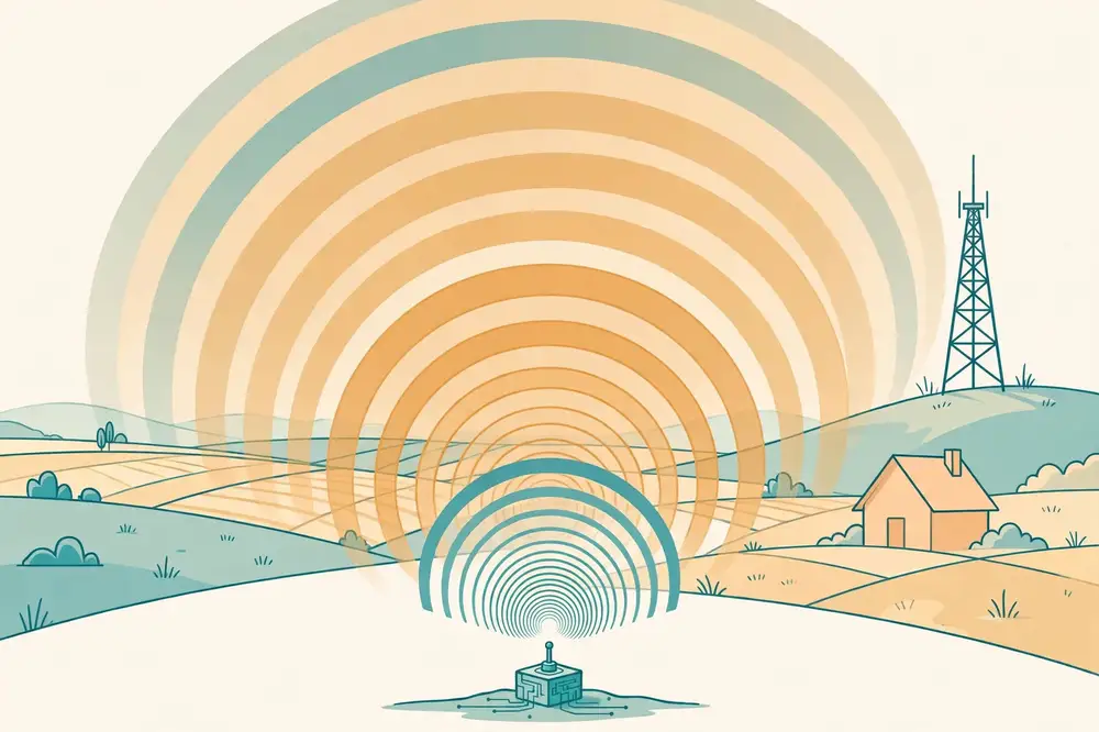
Every wireless choice trades off three things — you can optimize two, never all three:

Range: how far the signal usefully travels (meters to kilometers).
Power: how much energy each transmission costs (microwatts to watts).
Data rate: how much data per second (bits/sec to hundreds of Mb/s).

High data rate over long range costs power. Long range on tiny power means tiny data rates. Short range can be fast and cheap. This triangle explains the entire connectivity landscape: each technology is a different point on it, and your research deployment must pick the point that matches the physical reality of your site. A farm with no Wi-Fi 2 km from the nearest building simply cannot use Wi-Fi — physics decides, not preference.

5.2 The technologies

Wi-Fi (IEEE 802.11)

The familiar standard. High data rates (tens to hundreds of Mb/s), range of tens of meters indoors (up to ~100 m line-of-sight outdoors), and high power draw — an ESP32 transmitting Wi-Fi pulls 100–200+ mA. Use when: mains power is available, data volumes are large (images, audio), and an access point exists nearby. Avoid when: battery-powered nodes must last months, or distances exceed ~100 m. For research: Wi-Fi is perfect for lab prototypes and building deployments, and a poor choice for field sensor networks. Note that Wi-Fi association and DHCP take seconds and significant energy — a major cost in sleep/wake cycles.

Bluetooth / BLE (Bluetooth Low Energy)

Classic Bluetooth streams audio; BLE is the IoT-relevant variant — designed for tiny, infrequent data exchanges (sensor readings, beacons) at very low power, over ~10–50 m. A BLE sensor can run a year on a coin cell. Use when: a phone or gateway is nearby to collect data (wearables, indoor asset tags, phone-configured devices). BLE mesh extends coverage across a building. Avoid when: you need internet backhaul directly (BLE needs a gateway) or kilometer ranges.

LoRa and LoRaWAN

LoRa is a radio modulation technique (chirp spread spectrum) that achieves kilometers of range at milliwatts of power, at the cost of very low data rates (hundreds of bits/sec to ~tens of kb/s) and regulatory duty-cycle limits (in many regions, a device may transmit only ~1% of the time). LoRaWAN is the network protocol built on LoRa: end devices → gateways → network server → application server, with AES-128 encryption built in.

Use when: battery nodes spread over kilometers with tiny payloads (a 10-byte soil reading every 15 minutes is the canonical LoRaWAN application), especially where no Wi-Fi or cellular coverage exists. A single gateway can cover a village or a large farm. Avoid when: you need frequent updates, large payloads, or real-time control — LoRaWAN downlinks are limited and slow. Research gold: LoRaWAN deployments produce excellent papers on coverage mapping, energy measurement, and duty-cycle-compliant scheduling.

Zigbee (IEEE 802.15.4)

A low-power mesh networking standard: devices relay each other's messages, so the network heals around failures and extends range hop by hop. Data rates ~250 kb/s, range ~10–100 m per hop. Use when: dense indoor deployments (smart buildings, greenhouses) where mains-powered devices can act as always-on routers. Avoid when: nodes are sparse (mesh needs density) or all nodes are battery-powered (someone must stay awake to route).

Cellular (2G/4G LTE, NB-IoT, LTE-M)

Cellular gives you the mobile network as backhaul — range wherever there is coverage, at the cost of a SIM/subscription and higher power (though NB-IoT and LTE-M are low-power variants designed for IoT: small data, deep sleep, years on battery where coverage exists). Use when: nodes are far apart, mobile coverage exists, and you cannot install your own gateway (vehicle tracking, remote pipeline monitoring). Avoid when: there is no coverage, subscription cost × hundreds of nodes breaks the budget, or power budget is extremely tight.

5.3 The comparison table (your site survey in one page)

Technology	Typical range	Data rate	Power profile	Topology	Best research use
Wi-Fi	~50–100 m	10s–100s Mb/s	High (100s mA TX)	Star (via AP)	Lab/building prototypes, image data
BLE	~10–50 m	~1 Mb/s	Very low (coin-cell years)	Star/mesh, needs gateway	Wearables, phone-adjacent sensing
LoRaWAN	2–15 km (rural–urban)	0.3–50 kb/s	Very low (years on battery)	Star-of-stars via gateways	Farms, villages, environmental monitoring
Zigbee	10–100 m/hop (mesh)	250 kb/s	Low (routers need mains)	Mesh	Dense indoor/greenhouse networks
Cellular NB-IoT/LTE-M	km (carrier coverage)	~100s kb/s	Low–medium	Star via carrier	Remote sites with coverage, no gateway option

Ranges are environment-dependent: walls, vegetation, and interference shrink them dramatically. Always do a site survey — walk the site with a test node and log signal strength (RSSI) at planned locations — before finalizing a deployment. "It worked on my desk" is the most expensive sentence in IoT research.

5.4 Network topologies

Star: every node talks directly to one central point (Wi-Fi AP, LoRaWAN gateway, cellular tower). Simple, but the center is a single point of failure and must be within range of all nodes.
Mesh: nodes relay for each other (Zigbee, BLE mesh). Self-healing and extendable, but routing costs energy and complexity.
Star-of-stars (LoRaWAN): nodes → multiple gateways → network server. Nodes don't associate with a specific gateway; any gateway in range forwards. Elegant for wide-area coverage.

5.5 A connectivity decision walkthrough

Scenario: soil-moisture monitoring across a 2 km² farm, readings every 15 minutes, no mains power, no Wi-Fi, patchy cellular coverage.

Data size: 10 bytes per reading — tiny. Eliminates nothing yet, but favors low-rate options.
Range: 2 km, no infrastructure → Wi-Fi, BLE, Zigbee eliminated (range). Left: LoRaWAN, cellular.
Power: battery for a growing season → both possible, LoRaWAN better.
Coverage: patchy cellular → risky; LoRaWAN lets you install your own gateway on a farmhouse roof.
Cost: one gateway + cheap nodes vs per-node SIM subscriptions → LoRaWAN wins.

Decision: LoRaWAN. Document this reasoning chain in your thesis — it is exactly the analysis reviewers expect, and it generalizes to any deployment.

5.6 Deep dive: LoRa spreading factors and LoRaWAN device classes

LoRa's range-vs-rate trade-off is tunable via the spreading factor (SF7–SF12): higher SF = longer range and better obstacle penetration, but ~2× the airtime per step up. Airtime matters because (a) it costs energy and (b) regulations in many regions cap duty cycle at 1% — at SF12, a single 50-byte message can take over a second of airtime, limiting you to a handful of messages per hour. Adaptive Data Rate (ADR) lets the network server automatically step each device down to the fastest SF its link supports — always enable ADR for stationary nodes; it is free energy savings.

LoRaWAN device classes define downlink behavior:

Class A (default): device-initiated; after each uplink, two short receive windows open for downlinks. Lowest power — the right choice for sensors.
Class B: adds scheduled receive windows (beaconed) — for devices needing regular downlinks at known times.
Class C: receive window nearly always open — for mains-powered actuators needing instant commands, at high energy cost.

Most research sensor nodes are Class A. If your experiment needs commands to battery devices (actuation over LoRaWAN), understand that Class A downlinks only arrive right after uplinks — control latency equals your uplink interval. Design the control law around that.

5.7 Deep dive: link budgets and why "up to 15 km" is a lie indoors

Radio range claims assume ideal conditions. The link budget — transmit power + antenna gains − path loss − margins — determines reality, and path loss grows with the square of distance (worse with obstacles: a single concrete wall can cost 10–20 dB, equivalent to ~10× the distance in free space). Practical consequences:

Antenna matters enormously: the tiny PCB antenna on a cheap module vs a proper external antenna can be the difference between working and dead at 500 m. Keep antennas vertical, clear of metal, and away from the PCB ground plane.
Height is range: raising a gateway from 2 m to 10 m often doubles useful coverage (Fresnel zone clearance). Gateway placement is a deployment decision worth a site visit.
Measure, don't assume: log RSSI and SNR with every message (Chapter 8's metadata rule). SNR below ~−10 dB on LoRa means you're near the edge; Wi-Fi RSSI below −80 dBm means trouble. A coverage heatmap from real measurements is publishable data.

5.8 Cellular IoT: NB-IoT vs LTE-M vs 4G

NB-IoT: 180 kHz bandwidth, ~250 kb/s peak, excellent building penetration and battery life (PSM/eDRX sleep modes give 10-year claims), but no mobility handover and high latency — for stationary sensors.
LTE-M: 1.4 MHz, ~1 Mb/s, supports mobility and voice — for trackers and vehicles.
Standard 4G LTE: full speed, full power — for gateways and cameras, with a router, not a sensor node.

The catch for researchers: module cost ($15–40), SIM/data-plan logistics per node, and carrier sunsets (2G/3G shutdowns have orphaned deployments — never design around a network generation being phased out). Where coverage is good and node count is low, cellular is the fastest path to a working wide-area deployment: no gateway to install, no duty-cycle limits.

5.9 Emerging options: 5G RedCap, Wi-Fi HaLow, satellite

Know what's on the horizon, and when to care:

5G RedCap (Reduced Capability): a mid-tier 5G profile — more capable than NB-IoT, far less power-hungry than full 5G. Relevant for video-capable IoT (cameras, drones) where LTE is being sunset. For typical sensor theses: watch, don't adopt yet.
Wi-Fi HaLow (802.11ah): Wi-Fi on sub-1 GHz — ~1 km range, low power, IP-native. Technically lovely for campus/farm sensor networks; ecosystem still maturing. A reasonable thesis topic is evaluating HaLow against LoRaWAN on real hardware.
Satellite IoT (e.g., Swarm/Lacuna-style store-and-forward, 3GPP NTN): for truly remote sites (ocean buoys, desert stations) — tiny messages, high latency, per-message cost. Only when nothing terrestrial reaches.
Matter/Thread: the smart-home interoperability push (Thread = 802.15.4 mesh with IPv6). Relevant if your research touches consumer smart-home devices.

The pattern: adopt proven technology for the thesis deployment, and relegate emerging tech to the "future work" section — unless the emerging tech is your research question.

For your research: Connectivity choice is one of the most defensible "engineering contribution" sections in an IoT thesis. Measure and report: RSSI/SNR at deployment points, packet delivery ratio over at least a week, and energy per transmission. A table of measured link quality across your site is original data that no one else has — publishable in itself as part of a deployment paper.

Key takeaways:

Range, power, and data rate form an iron triangle — pick the technology whose corner matches your site.
Wi-Fi = fast but power-hungry and short-range; BLE = ultra-low-power near a phone/gateway; LoRaWAN = kilometers on batteries for tiny payloads; Zigbee = indoor mesh; cellular = carrier coverage at subscription cost.
Do a site survey with RSSI logging before committing; desk tests do not transfer to the field.
Write down your connectivity decision chain — it is a core part of your methodology.

Chapter 6: Protocols — MQTT, HTTP, CoAP

6.1 Why protocols matter

Connectivity (Chapter 5) moves bits through the air. Protocols define what the bits mean — how devices address each other, how messages are structured, and what delivery guarantees exist. Choosing the wrong protocol wastes power, breaks at scale, or makes your data model unmanageable. For IoT, three application protocols cover nearly everything: MQTT, HTTP, and CoAP.

6.2 MQTT: publish/subscribe, deeply explained

MQTT (MQ Telemetry Transport, standardized by OASIS and ISO/IEC 20922) is the dominant IoT messaging protocol, and understanding it deeply pays off across your whole research career. Its core idea is publish/subscribe with a broker:

Clients (sensors, dashboards, backend services) connect to a central broker.
A client publishes messages to a topic — a hierarchical string like farm/plot-3/soil-moisture.
Other clients subscribe to topics (exact or with wildcards: farm/+/soil-moisture subscribes to all plots; farm/# subscribes to everything under farm/).
The broker routes each published message to all matching subscribers.

Why this design is brilliant for IoT:

Decoupling. Publishers don't know who subscribes, and vice versa. Add a new dashboard or alerting service without touching a single sensor node. Your field nodes and your analysis code evolve independently — essential for long research deployments.
Tiny overhead. An MQTT packet header can be as small as 2 bytes. On a LoRa or battery budget, every byte costs energy; MQTT was designed for exactly this constraint.
Persistent connections. The device holds one TCP connection open and pushes data when ready, instead of repeatedly opening connections (HTTP's expensive habit). This is dramatically more energy-efficient for frequent small messages.
Quality of Service (QoS) levels — the delivery contract, and a favorite exam/reviewer question:
QoS 0 — at most once: fire and forget. Fastest, cheapest; messages can be lost. Fine for routine sensor readings where the next reading comes in a minute anyway.
QoS 1 — at least once: the broker acknowledges; the sender retries until acknowledged. Guaranteed delivery, but duplicates possible — your backend must handle duplicates (idempotency).
QoS 2 — exactly once: a four-step handshake guarantees single delivery. Safest, most expensive in energy and latency. Reserve for commands that must not duplicate (unlock a door, dispense medicine).
Retained messages: the broker stores the last message on a topic and delivers it immediately to new subscribers — so a dashboard that connects at noon instantly sees the latest soil reading from 11:45, not a blank screen.
Last Will and Testament (LWT): on connecting, a device registers a "will" message ("node-7 offline") that the broker publishes automatically if the device disconnects unexpectedly. This is how dashboards show honest online/offline status instead of frozen stale data.
Sessions: persistent sessions let the broker queue messages for a sleeping subscriber and deliver on reconnect — tailor-made for battery nodes that wake briefly.

A data-flow walkthrough — the full MQTT journey of one reading:

ESP32 wakes, reads soil moisture: 34%.
It publishes {"moisture": 34, "ts": "2026-10-08T06:15:00Z", "battery": 3.9} to topic farm/plot-3/soil-moisture at QoS 1.
The broker (e.g., Mosquitto, or a cloud broker) acknowledges receipt (QoS 1 handshake).
The broker forwards the message to all subscribers: the time-series database ingester (subscribed to farm/#), the dashboard backend, and the alerting service (subscribed to farm/+/soil-moisture).
The alerting service sees 34% > threshold 30% → no action. Had it been 25%, it would publish a command to farm/plot-3/pump/set → the node's subscription receives it → pump starts.
The ESP32 returns to deep sleep. Total airtime: a fraction of a second.

Notice the topic design carries your data model: site/plot/metric hierarchies with wildcards are the standard pattern. Design topics before you deploy; renaming topics mid-experiment breaks subscribers.

6.3 HTTP: the familiar workhorse

HTTP (usually with REST APIs and JSON) is request/response: the device opens a connection, POSTs data to a URL, gets a response, closes. Every web developer knows it, every cloud platform accepts it, and debugging is trivial (curl, browser dev tools).

Trade-offs: each request carries large headers (hundreds of bytes — often bigger than the sensor payload itself), and establishing TLS + TCP connections costs seconds and significant energy. For a mains-powered gateway sending batches every minute, HTTP is perfectly fine. For a battery node sending 10 bytes every 15 minutes, HTTP's overhead can dominate the energy budget. Also, HTTP is client-initiated only — the server cannot push a command to the device without polling or workarounds (websockets, long polling), whereas MQTT subscriptions deliver commands naturally.

Rule of thumb: HTTP for gateway-to-cloud and dashboard APIs; MQTT for device-to-platform messaging.

6.4 CoAP: MQTT's lightweight cousin

CoAP (Constrained Application Protocol, IETF RFC 7252) is essentially "HTTP ideas redesigned for tiny devices": it uses UDP instead of TCP (no connection setup — big energy saving), supports GET/POST/PUT/DELETE semantics on resources (like REST), and adds an observe mode where a client subscribes to resource changes (like publish/subscribe). Message overhead is ~4 bytes.

Use when: extremely constrained devices/networks (6LoWPAN meshes, NB-IoT) where even MQTT's TCP connection is too heavy. Reality check: CoAP has a smaller ecosystem than MQTT — fewer brokers, fewer tutorials, fewer managed services. For most student research, MQTT's ecosystem advantage outweighs CoAP's technical elegance. Know CoAP exists, know why (UDP, observe), and reach for it only when measurements prove you need it.

6.5 Protocol chooser

Need	Choice	Why
Battery nodes, frequent small messages, commands to devices	MQTT	Tiny overhead, persistent connection, pub/sub, QoS, LWT
Gateway → cloud batch uploads, dashboard APIs	HTTP/REST	Universal, debuggable, fine on mains power
Ultra-constrained UDP networks, REST-like semantics	CoAP	4-byte header, observe mode; smaller ecosystem
Must never lose a reading	MQTT QoS 1 (+ idempotent backend)	Retries with dedup logic
Must never duplicate a command	MQTT QoS 2	Exactly-once handshake
Dashboard needs latest value on connect	MQTT retained messages	Broker replays last value

Security note (expanded in Chapter 9): MQTT without TLS sends credentials and data in cleartext. Always use TLS (port 8883), unique per-device credentials or certificates, and topic ACLs so a compromised node can't publish to another node's command topics.

6.6 Deep dive: MQTT brokers and MQTT v5

Choosing a broker: Eclipse Mosquitto is the open-source default — tiny, runs on a Raspberry Pi, perfect for research. EMQX and HiveMQ add clustering and management UIs for larger deployments. Cloud providers offer managed brokers (verify current offerings before committing a thesis to one — managed IoT services have been discontinued before). For a thesis, self-hosted Mosquitto on your gateway keeps you independent of cloud pricing changes and gives you full log access for analysis.

MQTT v5 (the current standard) adds features worth knowing: reason codes on every acknowledgment (so you can distinguish "rejected: quota exceeded" from "rejected: not authorized" in logs), topic aliases (numeric shortcuts that shrink repeated topic strings — real bandwidth savings on constrained links), message expiry (stale sensor data auto-discarded by the broker), request/response patterns, and shared subscriptions (a $share/group/topic subscription distributes messages across multiple consumers — load balancing for your ingestion workers). You can do excellent research on MQTT v3.1.1, but cite v5 as the current standard.

MQTT-SN (Sensor Networks) adapts MQTT to UDP/non-TCP transports for the most constrained devices — know it exists; you will rarely need it with ESP32-class hardware.

6.7 Topic design: patterns and anti-patterns

Good topic hierarchies share traits: fixed depth (site/device/metric), no spaces or wildcards in published topics, device ID included (so you can trace every message to its source), and separate namespaces for telemetry vs commands (…/telemetry/ vs …/cmd/) so ACLs are simple.

Anti-patterns seen in failed deployments: encoding the value in the topic (farm/temp/25.3 — topics are addresses, not data), one giant flat namespace with no hierarchy (unsubscribable), and changing topic structure mid-deployment (version your topics: v1/farm/… if you expect evolution). Write the topic schema in a one-page document before flashing the first node — it is a contract between your firmware team (you) and your backend team (also you, next month).

6.8 When not to use MQTT

Honest engineering names the limits: for request/response RPC between services, HTTP is more natural; for high-throughput streaming (video, bulk transfer), dedicated streaming or file transfer wins; for browser-to-device direct control, MQTT-over-WebSockets bridges the gap (and is how web dashboards subscribe live). MQTT dominates device-to-platform telemetry — use the right tool elsewhere.

6.9 Payload formats: JSON vs binary

The examples in this book use JSON — human-readable, debuggable, universally supported. Its cost: verbosity. A 60-byte JSON reading might be 12 bytes in a binary format. Options:

JSON: default choice. Readable in logs, trivial to parse everywhere. Use it unless measurements say otherwise.
CBOR (Concise Binary Object Representation, RFC 8949): JSON's data model in binary — ~40–60% smaller, still self-describing. The natural upgrade for constrained links; CoAP's native partner.
Protocol Buffers / custom binary: smallest, fastest — but needs a shared schema and custom tooling on both ends. Worth it for LoRaWAN-scale constraints or very high message rates.

Rule: start with JSON, measure the energy/bandwidth cost, and switch to CBOR only if the numbers justify the debugging pain. A thesis that reports "switching payloads from JSON to CBOR cut airtime by 45% and extended battery life 12%" is a clean, honest contribution. Also consider SenML (Sensor Measurement Lists, RFC 8428) — a standard JSON/CBOR format for sensor data with units and timestamps built in. Using a standard format makes your dataset interoperable and your methodology section shorter.

6.10 Lab practice: running your own broker in ten minutes

Theory sticks when you touch it. On any Linux machine (or Raspberry Pi):

Install Mosquitto (apt install mosquitto mosquitto-clients).
In one terminal, subscribe: mosquitto_sub -h localhost -t 'lab/#' -v — this prints every message under lab/.
In another, publish: mosquitto_pub -h localhost -t 'lab/node-1/temp' -m '{"t": 24.6}'.
Watch the message arrive. Now publish with -r (retained), kill the subscriber, resubscribe — the retained message replays instantly. Publish a second message to lab/node-1/temp and a third to lab/node-2/temp, then subscribe to lab/+/temp — the + wildcard matches one level. Then lab/# — # matches everything below.

Extend it: enable authentication (a password file), then TLS with a self-signed certificate, and observe what breaks at each step — that breakage is the curriculum. Every concept in this chapter (topics, wildcards, retained, QoS, auth, TLS) becomes concrete in under an hour, and the exact commands belong in your lab notebook for when you configure the field gateway.

For your research: Your protocol choice, QoS selection, and topic hierarchy belong in the methodology chapter with one paragraph of justification each. A strong, publishable mini-study: measure energy per message for MQTT (QoS 0 vs 1) versus HTTP POST on your actual hardware, and report the numbers — this is original, useful, and frequently cited data.

Key takeaways:

MQTT's brokered publish/subscribe decouples producers from consumers; topics with wildcards are your data model — design them first.
QoS 0 = fire-and-forget, QoS 1 = at-least-once (handle duplicates), QoS 2 = exactly-once (for critical commands).
Retained messages solve the "blank dashboard" problem; Last Will gives honest offline detection.
HTTP for gateways and APIs; MQTT for devices; CoAP when UDP-level constraints demand it. Always run MQTT over TLS with per-device credentials.

End of chunk 2 of 4 — continues with Chapters 7–9.

Chapter 7: Edge vs Cloud — Where Should Computing Happen?

7.1 The spectrum, not a binary

"Edge vs cloud" is often presented as a choice between two boxes. In reality it is a spectrum of where computation happens, measured by distance from the sensor:

On-device (tiny edge): the microcontroller itself — threshold checks, filtering, TinyML inference.
Gateway edge: a Raspberry Pi or industrial gateway near the devices — aggregation, local dashboards, protocol translation, buffering during outages.
Cloud: remote data centers — long-term storage, heavy analytics, training ML models, global dashboards.

The right answer for each piece of logic is the closest place that can do the job reliably. Push work as close to the sensor as the hardware allows; pull it toward the cloud only when edge resources are insufficient. This principle — compute at the lowest capable layer — resolves most edge/cloud debates.

7.2 What the edge is good at

Latency: a greenhouse vent that must open within a second of a temperature spike cannot wait for a cloud round-trip (especially over LoRaWAN, where a downlink can take seconds to minutes). Control loops live at the edge.
Offline resilience: farms, factories, and remote sites lose connectivity. An edge gateway keeps logging locally and syncs when the link returns — your dataset gets no gaps.
Bandwidth and cost savings: a camera sending 24/7 video to the cloud is ruinously expensive; an edge device that sends only "intruder detected" events plus a snapshot is cheap. Rule of thumb: send insights, not raw streams.
Privacy: health and human-monitoring data processed on-device never traverses the internet — easier ethics approval, easier GDPR-style compliance.

7.3 What the cloud is good at

Scale and elasticity: storing years of data from thousands of nodes, running queries over all of it, training ML models on GPUs.
Accessibility: dashboards and APIs reachable from anywhere, managed backups, managed MQTT brokers and time-series databases you don't have to babysit.
Heavy computation: model training, large-scale aggregation, cross-site analytics — workloads no microcontroller or Pi can touch.

7.4 Decision framework

Factor	Favors edge	Favors cloud
Response time needed	< 1 s, or control loop	Minutes to hours acceptable
Connectivity	Intermittent or expensive	Reliable and cheap
Data volume	High raw volume, low insight density (video, vibration)	Small, structured readings
Compute need	Simple rules, thresholds, tiny models	Training, large joins, complex analytics
Privacy sensitivity	Personal/health data	Aggregated, anonymized data
Power	Mains-powered gateway available	Battery nodes only (keep them dumb, compute centrally)

Worked example — air-quality research station: The node (ESP32 + PMS5003 + SCD30) computes 5-minute medians on-device (rejects outliers, saves power by transmitting summaries — edge). A Raspberry Pi gateway collects from 10 nodes, stores to a local database, serves a local dashboard, and syncs hourly to the cloud (gateway edge). The cloud holds the full multi-month dataset, runs calibration models against the reference station, and hosts the public dashboard (cloud). Each layer does what it's best at — and the thesis can describe this cleanly.

7.5 TinyML: machine learning on microcontrollers

TinyML is the practice of running small neural networks directly on microcontrollers (tens of KB of RAM). Frameworks like TensorFlow Lite for Microcontrollers let you deploy models that do keyword spotting, anomaly detection on vibration data, or simple image classification on devices like the ESP32. The workflow: train in the cloud on collected data → quantize/compress the model → deploy to the MCU → run inference locally, sending only results.

For researchers, TinyML is attractive because it turns a data collection project into a smart sensing project — a publishable step up. But be honest about limits: MCU models are small, accuracy is bounded, and evaluation must be on real device-collected data, not just lab datasets.

7.6 Fog computing (know the term)

Fog is sometimes used for the layer between edge and cloud — regional servers, on-premise clusters. In practice, most student work needs only the three tiers above. If a paper says "fog," mentally map it to "gateway/regional edge" and move on.

7.7 Deep dive: the gateway software stack

A Raspberry Pi gateway typically runs a small constellation of services — learn the standard pieces:

Mosquitto (MQTT broker) — the message hub.
Node-RED — a visual flow-based tool for wiring logic: "when MQTT topic X exceeds threshold, send email and write to database." Invaluable for prototyping gateway logic without writing backend code; many theses use it as the actual (not just prototype) rules engine.
InfluxDB/TimescaleDB — time-series storage.
Grafana — dashboards and alerting.
A sync agent — rsync, or a small script that replays buffered data to the cloud when connectivity returns.

All five run comfortably on one Pi for tens of nodes. Deploy them with Docker Compose — one YAML file defines the whole stack, making your setup reproducible and your methodology's "system setup" section a single code listing. Reproducibility is a research virtue; a compose file is reproducibility you can download.

7.8 Deep dive: TinyML workflow in practice

The TinyML pipeline, concretely:

Collect labeled data from your actual sensors (e.g., 500 vibration samples: normal vs bearing-fault).
Train a small model (a tiny neural net or even a decision tree) in Python on your laptop/cloud.
Quantize — convert 32-bit floats to 8-bit integers. This shrinks the model ~4× with typically 1–3% accuracy loss; TensorFlow Lite for Microcontrollers and Edge Impulse (a managed TinyML platform popular in research) automate this.
Deploy the resulting C array to the ESP32; run inference in the loop.
Evaluate on-device — measure accuracy and inference time and energy per inference on the real board, not just in simulation.

The research contribution is usually in step 5's honest measurement or in making the model smaller without losing accuracy (pruning, quantization studies). A keyword-spotting or anomaly-detection demo that reports only lab accuracy is a demo; one that reports on-device latency, RAM, and energy is a paper.

7.9 Measuring what matters: latency budgets

"Edge is faster" is a slogan; a latency budget is engineering. Break end-to-end latency into components and measure each: sensor acquisition time + on-device processing + transmission airtime + network transit + broker routing + backend processing + dashboard render. For a LoRaWAN Class A control loop, the dominant term is often the downlink wait (up to your uplink interval) — which no amount of cloud optimization fixes. Measure the budget for your critical loop, publish the breakdown, and place computation to attack the biggest term. This is the kind of figure reviewers remember.

7.10 Cost modeling: the other half of the decision

Latency and reliability get the attention, but cost decides deployments. Model total cost of ownership (TCO) over the deployment lifetime:

Cloud costs: managed broker messages/month, database storage and queries, egress bandwidth, dashboard users. A "free tier" that covers your pilot can become a real bill at 100 nodes — price the full deployment, not the demo.
Edge costs: gateway hardware (one-time), power, physical maintenance visits (the dominant cost in remote deployments — a site visit can cost more than the node).
Connectivity costs: SIM subscriptions × nodes × months vs one LoRaWAN gateway (one-time) vs existing Wi-Fi (free but not yours to rely on).

A simple TCO table (3-year horizon, per-node and total) belongs in any deployment paper's discussion — and often the conclusion surprises: for the greenhouse capstone, the self-hosted Pi stack costs ~$70 once versus managed-cloud fees that exceed it within a year at scale. For a 5-node pilot, the cloud wins on convenience. State the crossover point; that's analysis, not opinion.

7.11 Case study: the same system, two placements

Consider a vibration-monitoring node on factory motors, sampling at 1 kHz to detect bearing faults:

Placement A (cloud): stream raw vibration to the cloud; run FFT + classifier there. Bandwidth: ~86 M samples/day/node — prohibitive over any wireless link; latency to alert: seconds; works only with wired Ethernet.
Placement B (edge): compute FFT on the ESP32, run a tiny anomaly model, transmit only spectral features + alerts (a few hundred bytes/hour). Bandwidth: trivial; latency: milliseconds; runs on Wi-Fi or even LoRaWAN.

Placement B is the only feasible wireless design — and the thesis writes itself: on-device FFT accuracy vs cloud FFT accuracy (quantization effects), energy per inference, and alert latency. Whenever someone proposes "just send it to the cloud," ask for the bandwidth math first.

7.12 Decision worksheet: scoring a placement

When the choice isn't obvious, score it. List candidate placements as rows, decision factors as columns, weight what matters:

Factor (weight)	On-device	Gateway	Cloud
Latency need: <1 s (×3)	9	6	2
Works offline (×3)	9	8	1
Compute adequate (×2)	3	7	9
Bandwidth cost (×2)	9	7	3
Dev effort (×1)	4	6	8
Weighted total	70	71	48

(Scores 1–9 per cell; totals illustrative.) The worksheet's value isn't the winner — it's forcing you to name factors and weights explicitly, which is exactly what your methodology's architecture justification should contain. Different deployments weight differently: a hospital monitor weights latency and offline at ×5; a climate archive weights compute and storage. Show your weights; defend them in one paragraph each.

7.13 The hybrid reality: most systems use all three tiers

Purist "all edge" or "all cloud" designs are rare in practice. The greenhouse capstone (Chapter 12) is typical: threshold control on the ESP32 (tier 1 — must work during outages), aggregation, storage, and dashboard on the Pi gateway (tier 2 — the offline-capable core), and nightly cloud backup plus heavy analysis on a server (tier 3 — scale and convenience). When you draw your architecture, expect arrows at every tier boundary and label what crosses each one (raw readings up, aggregates up, commands down, backups up). A reviewer who sees a thoughtful hybrid with justified boundaries reads "systems thinker"; a reviewer who sees everything crammed into one tier reads "demo." Design for the hybrid from the start — retrofitting a tier boundary into finished firmware is painful.

For your research: Draw your system's compute placement as a diagram with one sentence of justification per component ("thresholding on-device to guarantee <1 s response during connectivity outages"). Reviewers treat this as evidence of systems thinking. An excellent thesis contribution: measure the same pipeline's latency, bandwidth, and energy at two placements (e.g., raw-data-to-cloud vs edge-aggregated) and report the trade-off curve.

Key takeaways:

Edge vs cloud is a spectrum: on-device → gateway → cloud. Compute at the lowest capable layer.
Edge wins on latency, offline resilience, bandwidth savings, and privacy; cloud wins on scale, heavy compute, and accessibility.
Send insights, not raw streams — aggregation at the edge is the single biggest cost saver.
TinyML lets microcontrollers run small models locally; train in cloud, infer at edge.

Chapter 8: IoT Data Pipelines — From Sensor to Dashboard

IoT data pipeline flow

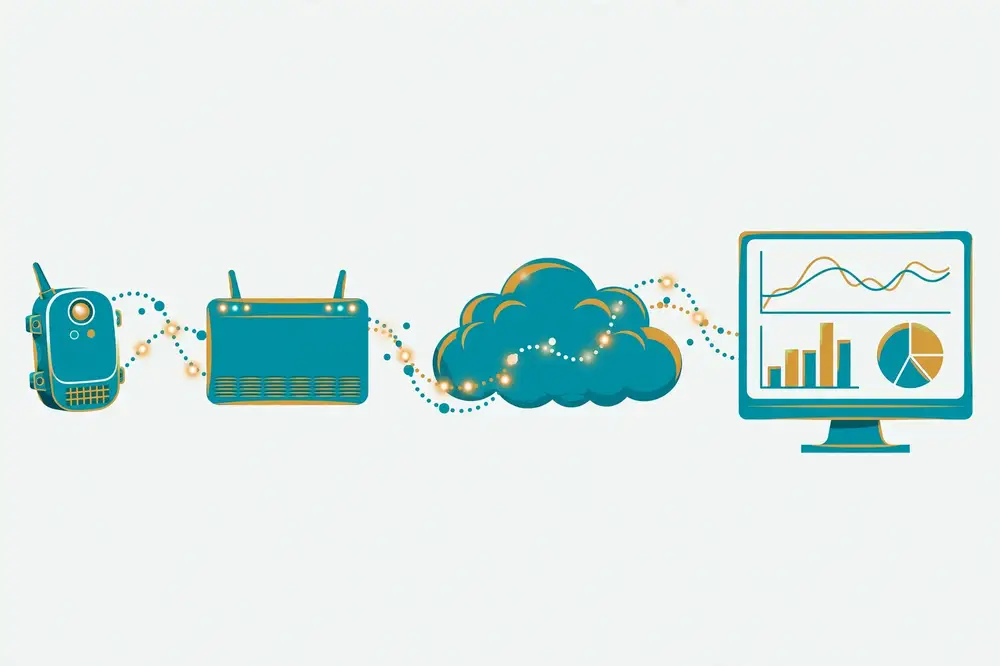
8.1 The pipeline, end to end

A single sensor reading travels a long road before it becomes a dot on a chart. Trace it once, completely, and you will never be confused by IoT architecture diagrams again:

Sense: the physical quantity becomes an electrical signal (Chapter 2).
Digitize & calibrate: ADC → raw number → calibrated value via the sensor's formula.
Timestamp: attach the time of measurement. This is more important than beginners think — without trustworthy timestamps, your data is a pile of numbers, not a time series.
Buffer locally: store readings in flash/RAM so nothing is lost during network outages.
Transmit: send via the chosen connectivity and protocol (Chapters 5–6).
Ingest: the broker/backend receives, validates (range checks, schema checks), and deduplicates.
Store: write to a time-series database (TSDB) — databases optimized for timestamped data (InfluxDB, TimescaleDB, or even PostgreSQL with the Timescale extension).
Process: clean, aggregate (minute/hourly means), join with other sources, run detection rules or models.
Serve: dashboards (Grafana is the open-source standard), APIs, alerts (SMS/email), and exports for analysis.

Every stage can fail, and each failure has a characteristic symptom — learn the mapping: gaps in data → buffering/transmission; wrong values → calibration; wrong times → clock sync; duplicates → QoS retries without dedup; dashboard blank after reconnect → no retained messages.

8.2 Time: the hidden hard problem

Microcontrollers have no real clock — they count milliseconds since boot. For research data, you need wall-clock time, and there are three standard approaches:

NTP (Network Time Protocol): over Wi-Fi/cellular, the device asks internet time servers. Accurate to tens of milliseconds; costs a network transaction at boot and periodically.
RTC (real-time clock) modules (e.g., DS3231): a battery-backed chip that keeps time through power loss, accurate to ~a minute per year. Essential for offline/log-first devices.
Network-provided time: LoRaWAN and cellular networks can provide timestamps; GPS modules give extremely accurate time (plus location) at high power cost.

Best practice: timestamp at the moment of measurement on the device (not when the server receives it — network delays of seconds to hours would corrupt your time axis), store in UTC (ISO 8601 format), and convert to local time only for display. Document your time source and its accuracy in the methodology.

8.3 Data formats and schemas

Keep payloads small, structured, and self-describing:

{
  "device_id": "node-07",
  "ts": "2026-10-08T06:15:00Z",
  "soil_moisture_pct": 34.2,
  "soil_temp_c": 24.8,
  "battery_v": 3.92,
  "rssi_dbm": -87
}

Include metadata with the data: device ID, timestamp, battery voltage, and signal strength (RSSI) in every message. When a sensor starts drifting six weeks into a deployment, the battery-voltage and RSSI columns are what let you diagnose it instead of guessing. This is the cheapest insurance in IoT research.

8.4 Storage: why time-series databases

A TSDB stores (timestamp, measurement, tags) efficiently and answers time-range queries fast: "hourly mean soil moisture for plot 3 in July" should return in milliseconds, not minutes. InfluxDB and TimescaleDB are the common open-source choices; both integrate with Grafana for dashboards. For a thesis-scale deployment (tens of nodes, months of data), a single Raspberry Pi can comfortably run all three — a fact that keeps research budgets sane.

Retention and downsampling: raw data accumulates fast. A common policy: keep raw readings for 90 days, keep hourly aggregates for 2 years, keep daily aggregates indefinitely. Define this before deploying, not after the disk fills.

8.5 Dashboards and alerts

Grafana is the standard: connect it to your TSDB, build time-series panels, set alert rules (e.g., "soil moisture < 30% for 2 hours → send email/SMS"). For public-facing or custom needs, a small web app (Python Flask/FastAPI, Node.js) reading from the database works. Whatever you build, include: live values with "last updated" timestamps (stale data must look stale), historical charts with zoom, and an honest device-status view (online/offline via MQTT Last Will, battery levels).

8.6 A pipeline walkthrough: the complete journey of one reading

Revisit the soil node, now with the full pipeline visible:

06:15:00 — capacitive probe read; ADC value 2,847 → calibration curve → 34.2% moisture.
Device clock (synced via NTP at boot, drift < 1 s/day) stamps 2026-10-08T06:15:00Z.
Reading appended to a local ring buffer in flash (holds 48 h of readings).
MQTT publish (QoS 1) to farm/plot-3/soil-moisture; broker acknowledges; buffer entry marked sent.
Ingestion service validates: moisture within 0–100%, timestamp within 24 h of now → accept.
Written to InfluxDB with tags plot=3, device=node-07.
A continuous query computes the hourly mean into a downsampled table.
Grafana shows the live chart; the alert rule watches the threshold; at 06:15 the value is fine — no alert.
Weekly, a script exports CSV for the researcher's analysis notebook.

If the network had been down at step 4, the reading would have waited in the buffer and been sent with its original timestamp when connectivity returned — no gap, no time corruption. That is what a well-built pipeline guarantees, and it is worth a paragraph in every IoT thesis.

8.7 Deep dive: ingestion — validation, dedup, and ordering

The ingestion service is where raw messages become trustworthy data. Build it as an explicit stage (a small Python/Node.js service subscribed to …/#), not as hope:

Schema validation: reject messages missing required fields or with wrong types. Log rejections with counts — a sudden spike in rejections is your first warning of a firmware bug or a dying sensor.
Range checks: per-sensor plausible ranges (soil moisture 0–100%, battery 3.0–4.2 V). Out-of-range values are quarantined, not silently stored.
Deduplication: QoS 1 retries and reconnect replays create duplicates. Dedup on (device_id, ts) — keep a short window of seen keys. Without this, your "hourly mean" double-counts.
Out-of-order handling: buffered replays arrive late. Your TSDB must accept out-of-order writes (InfluxDB and TimescaleDB both do), and your aggregation jobs must tolerate late data (recompute windows, or accept small corrections).
Backpressure: if the database slows, the ingester must queue rather than drop — a bounded in-memory queue spilling to disk. Size it for your worst outage.

A one-page description of this stage, with the validation rules listed, answers the reviewer's "how do you know the data is clean?" before they ask.

8.8 Deep dive: aggregation strategy and the "single pane" problem

Raw data answers "what happened at 06:15:00"; research answers "what happened this season." Bridge the gap with a deliberate aggregation strategy:

Continuous queries / downsampling tasks: precompute 5-min, hourly, and daily aggregates (mean, min, max, count) into separate tables. Dashboards query the aggregates (fast); analysts can still drill to raw (complete).
Event tables: control actions (pump ON/OFF), alerts, and maintenance events belong in their own tables with timestamps — joining events against sensor traces ("did irrigation actually raise moisture?") is the core analysis of control-system theses.
The single-pane rule: every number on your dashboard must be traceable to its source query. When a supervisor asks "where does this chart come from?", the answer is a query name, not a shrug.

8.9 Data dictionaries and dataset release

Research data outlives the project only if it's documented. Maintain a data dictionary from day one: every field name, unit, sensor model, calibration equation, and known quirk ("node-03's probe replaced 2026-11-02; offset +2.1% before"). When you release the dataset (and you should — released datasets are cited), package it as versioned CSV/Parquet + the dictionary + a README describing the deployment, following FAIR principles (Findable, Accessible, Interoperable, Reusable). A well-documented dataset from a student deployment routinely earns more citations than the paper that produced it.

8.10 Choosing your storage: a practical guide

Option	Strengths	Weaknesses	Use when
InfluxDB	Purpose-built TSDB, great Grafana integration, continuous queries	Query language (Flux/InfluxQL) learning curve; clustering is a paid feature	Default choice for sensor time series
TimescaleDB (PostgreSQL extension)	Full SQL, joins with relational data, hypertables	Heavier than InfluxDB for pure time series	You need SQL or mixed relational + series data
SQLite	Zero setup, single file, survives on tiny devices	No concurrent writers, weak for large scale	Single-node logging, prototypes
CSV files	Universal, human-readable, version-controllable	No indexing, slow queries, no types	Dataset release and interchange, not live storage

For a thesis: log to InfluxDB or TimescaleDB live, export versioned CSV/Parquet for analysis and release. Never analyze directly against the live database from a notebook — snapshot first, so your results are reproducible against a fixed dataset version.

8.11 Alerting done right

Alerts are where pipelines meet humans, and bad alerting destroys trust in the system:

Threshold + duration: alert when soil moisture < 30% for 2 consecutive readings, not on a single dip — single-reading alerts fire on noise and get ignored (alert fatigue).
Severity tiers: info (log it), warning (dashboard badge + email digest), critical (SMS/immediate). Define what each tier means before deployment.
Alert on the pipeline itself: "no data from node-07 for 1 hour" is often more important than any sensor threshold — silent nodes are failed nodes.
Rate limiting: one alert per condition per hour, with auto-resolve notifications ("moisture recovered to 46%"). Nobody reads the 47th identical SMS.

Grafana's alerting covers all of this with a few clicks — configure it on the gateway so alerts work even when the cloud link is down.

8.12 Schema evolution and backfill: planning for change

Your data model will change mid-deployment — a sensor gets added, a field gets renamed, a calibration equation updates. Plan for it:

Version your payloads: include "schema": 2 in the JSON. The ingester routes v1 and v2 through different parsers instead of crashing.
Never rewrite raw history: when calibration improves, write corrected values to a new table/column and keep the raw untouched. "We reprocessed with calibration v3" is reproducible; silently overwriting raw data is not.
Backfill procedure: when late/buffered data arrives, insert it into the raw table (TSDBs accept old timestamps), then re-run the aggregation jobs for the affected windows. Document the backfill in the dataset changelog.
Changelog: a simple CHANGELOG.md in your dataset repo — "2026-11-02: node-03 probe replaced; 2026-12-01: calibration v2 applied from this date" — is the difference between a dataset people trust and one they don't.

Deployments are living systems; the pipeline that assumes otherwise corrupts data quietly. Assume change, version everything, and keep raw data sacred.

For your research: Your thesis needs a pipeline diagram (like the one in this chapter's figure) with each stage labeled and the technology named at each stage. Then add a "failure handling" table: for each stage, what can fail and what your system does about it. This table is short to write and disproportionately impressive to reviewers — it proves you built a system, not a demo.

Key takeaways:

Trace every reading through nine stages: sense → digitize → timestamp → buffer → transmit → ingest → store → process → serve.
Timestamp at measurement time, in UTC; know your clock source and its accuracy.
Include metadata (device ID, battery, RSSI) in every payload — it is your future debugging lifeline.
Buffer locally and sync later: offline resilience is what separates deployments from demos.

Chapter 9: Security Basics for IoT

9.1 Why IoT security is uniquely hard

IoT devices are attractive targets and hard to defend: they are physically accessible (an attacker can steal or tamper with a field node), computationally weak (limited room for heavy cryptography), numerous (hundreds of identical devices = hundreds of identical attack surfaces), long-lived (deployed for years, rarely patched), and often built from default credentials and unencrypted protocols by developers in a hurry. High-profile incidents — from the Mirai botnet (2016), which hijacked hundreds of thousands of IoT devices with default passwords to launch record-breaking DDoS attacks, to compromised cameras and routers — all trace back to basics done wrong, not exotic zero-days.

For researchers, security matters twice: your deployment must not become someone else's attack infrastructure, and if your thesis involves human subjects (wearables, indoor monitoring), you carry ethical and legal obligations for their data.

9.2 The threat model: think like an attacker

Before choosing defenses, list what you are defending against — your threat model:

Threat	Example	Defense
Eavesdropping	Sniffing unencrypted MQTT to read farm data	TLS encryption in transit
Credential theft	Default passwords (admin/admin) on cameras/gateways	Unique strong credentials per device; no defaults
Device impersonation	Fake node injecting false sensor data	Per-device certificates or unique tokens; broker ACLs
Physical tampering	Stolen node, SD card read, sensor spoofing	Enclosures, encrypted storage where feasible, tamper-evident seals
Firmware attacks	Malicious OTA update	Signed firmware updates; secure boot on capable chips
Cloud/API attacks	Exposed dashboard with no login	Authentication, HTTPS, minimal exposed ports
Denial of service	Flooding the broker	Rate limiting, authentication, network segmentation

You do not need military-grade security; you need to close the cheap, well-known holes. Mirai succeeded because of default passwords — the fix was trivial and free.

9.3 The non-negotiable baseline (do all of these)

No default credentials. Every device, gateway, broker, and dashboard gets unique, strong credentials. This single step defeats the most common IoT attacks in existence.
Encrypt in transit. MQTT over TLS (port 8883), HTTPS for dashboards and APIs, never plaintext credentials on the wire.
Per-device identity. Each node gets its own credential/certificate — never one shared password for all nodes. When a node is compromised or retired, revoke just that one.
Least privilege (ACLs). A soil node may publish to farm/plot-3/# and subscribe to farm/plot-3/pump/set — and nothing else. A compromised node then cannot command other plots.
Keep software updated. Patch the gateway OS, the broker, and libraries. Plan an update mechanism before deployment; "we'll drive out and reflash" does not scale past ten nodes.
Secure the gateway. Change default OS passwords, disable unused services, firewall everything except what you need, use SSH keys instead of passwords.
Protect data at rest where sensitive: encrypted database volumes, encrypted backups.

If your IoT research involves people — occupancy sensors, wearables, cameras, microphones — additional obligations apply:

Informed consent: participants must understand what is collected, for how long, and for what purpose. Get ethics/IRB approval before deploying.
Data minimization: collect only what the research question needs. A presence study needs binary occupancy, not video.
Anonymization/pseudonymization: separate identities from measurements as early as possible; be aware that "anonymized" sensor traces can often be re-identified.
Retention limits: define and enforce a deletion schedule; "keep everything forever" is not an ethics-approved data plan.

9.5 Security in your thesis

Dedicate a short section to security: your threat model (a table like the one above, scoped to your deployment), the baseline measures you implemented, and known limitations ("nodes use TLS with per-device credentials; physical tamper resistance is limited to locked enclosures — acceptable because nodes are on private farmland"). Honest scoping impresses reviewers far more than claiming perfect security.

9.6 Deep dive: cryptography on constrained devices

You don't need to be a cryptographer, but you need to know what your devices can actually do:

TLS on ESP32: fully supported (mbedTLS in ESP-IDF / WiFiClientSecure in Arduino). The cost is real — handshake takes ~1–3 seconds and significant RAM — so use session resumption and keep connections persistent rather than reconnecting per message.
DTLS for UDP: CoAP-over-DTLS gives datagram security where TLS can't go. Heavier to implement; another reason MQTT-over-TLS is the pragmatic default.
X.509 certificates vs pre-shared keys: certificates scale better (per-device identity, easy revocation) but need provisioning infrastructure; pre-shared keys are simpler for small fleets. Either beats a shared password — pick one and document the provisioning process (how keys get onto devices securely at build time).
ESP32 flash encryption & secure boot: the chip supports encrypting flash contents and verifying firmware signatures at boot — enable both for field deployments. A stolen node then yields no credentials and runs no modified firmware. These are configuration options, not research projects; the research is in evaluating the overhead.
OTA updates: over-the-air firmware updates are essential past ~10 nodes, and they are the most dangerous feature you will build — an unsigned OTA channel is a remote-code-execution gift to attackers. Sign every image, verify the signature on-device before booting, and keep a rollback partition.

9.7 Network segmentation and the gateway as a firewall

Treat your IoT network as untrusted by default, even from your own LAN:

Put sensor nodes and the gateway on a separate VLAN/SSID from laptops and office systems, with firewall rules allowing only the gateway's required outbound connections.
The gateway exposes only what's needed: MQTT/TLS to nodes, HTTPS dashboard to users, SSH (key-only) to you. Everything else closed.
Log authentication failures on the broker and gateway; a simple daily "failed login attempts" line in your maintenance log catches scanning early.

This is standard IT hygiene applied to IoT — and its absence is the finding of half the IoT security audit papers ever published. Doing it in your deployment, and saying so, puts you ahead of most student work.

9.8 Incident response for tiny fleets

Write a one-page incident plan before deployment: how you revoke a compromised device's credentials (broker ACL + certificate revocation list), how you push an emergency firmware fix (signed OTA), who gets notified, and how you preserve logs for analysis. You will probably never use it — but the discipline of writing it forces you to verify that revocation and OTA actually work, which is the real value.

9.9 Case study: securing the greenhouse capstone

Apply the baseline (§9.3) to Chapter 12's greenhouse system, concretely:

Credentials: flash a unique MQTT username/password per ESP32 at build time (derived from the device ID + a secret you store offline); the Pi gateway uses an SSH key, password login disabled; Grafana behind HTTPS with individual accounts — no shared "admin/admin."
Transport: Mosquitto configured for TLS only (port 8883), with a self-signed CA you install on each node (document the CA rotation plan: 2-year expiry, rotation during a maintenance visit).
ACLs: acl_node-01 can publish greenhouse/bay-1/# and subscribe greenhouse/bay-1/cmd/# — nothing else. The ingestion service has read-only access to all telemetry; the dashboard backend can read but not publish commands; only the rules engine publishes to …/cmd/#.
Network: greenhouse Wi-Fi is a dedicated SSID/VLAN; the Pi's firewall allows 8883 (nodes), 443 (dashboard users), and SSH from your laptop's key only.
Updates: signed OTA via the gateway; firmware images versioned in git; a node that fails to boot the new image rolls back automatically (keep the known-good partition).
Physical: enclosures locked; nodes mounted out of casual reach; SD card on the Pi encrypted (LUKS) so a stolen gateway yields no credentials.

Write this as a half-page "security architecture" in your thesis — it answers the reviewer's security question completely, with specifics instead of slogans.

9.10 Testing your own security (ethically)

You may test your own deployment's security — and should, before a reviewer or attacker does:

Port scan the gateway (nmap) — you should see only the ports you intend.
Credential audit — try every default credential you can think of against your own devices; script it so it's repeatable.
Traffic sniffing — capture node traffic (Wireshark) and verify you cannot read credentials or payloads in plaintext.
Broker ACL test — connect as node-01 and try publishing to node-02's command topic; the broker must reject it.
Fuzz the ingestion — send malformed, oversized, and out-of-range payloads; the pipeline must reject them without crashing.

Document each test and its result in a table. "We attacked our own system and here is what held" is a strong, honest security section — and a fine standalone workshop paper.

9.11 Supply chain and firmware provenance

Your device's security starts before you unbox it:

Buy from reputable vendors. Counterfeit modules can carry modified firmware; for research deployments the risk is low but nonzero — and clone quality issues (§4.5) are the certain cost.
Verify firmware provenance: download toolchains and libraries from official sources, pin dependency versions, and keep a software bill of materials (SBOM) — a list of every library and version in your firmware. When a vulnerability is announced in a library you use, the SBOM tells you in seconds whether you're affected.
Build reproducibly: firmware built from a tagged git commit, with the commit hash logged at boot and transmitted in the metadata payload. When node-07 behaves oddly, the first question — "what firmware is it running?" — has an exact answer.
No secrets in source code: Wi-Fi passwords and API keys live in a separate, git-ignored config flashed at provisioning time — never in the repository, especially not a public one. Scan your repos before publishing; leaked credentials in GitHub student projects are depressingly common.

9.12 Privacy by design for sensor data

Even non-human deployments deserve privacy thinking, and human-adjacent ones require it:

Minimize at the source: if your research needs room occupancy, transmit a binary occupied/vacant flag — not audio, not video, not raw PIR waveforms that could be re-analyzed later for more than consented.
Aggregate early: a building study can publish floor-level aggregates while keeping room-level data restricted — decide the aggregation boundary in the ethics application, not after collection.
Separate identifiers from measurements as early in the pipeline as possible (pseudonymous device IDs mapped to identities only in a restricted lookup), and define who can access the mapping.
Plan deletion: "data will be deleted 2 years after publication" — and implement it. An unenforced retention policy is a fiction; schedule the deletion job.

Privacy designed in from the start is a paragraph in your ethics approval; privacy bolted on afterward is a rewrite of your pipeline.

For your research: A highly publishable contribution type is a security evaluation: take a common IoT setup (e.g., a popular tutorial's smart-home build), systematically test it against the baseline above, and report the gaps with fixes. Security-audit papers of real deployments are consistently accepted because they are useful, reproducible, and honest about limitations.

Key takeaways:

IoT's biggest breaches came from basics: default passwords and unencrypted traffic. Fix the basics first.
Build a threat model table, then apply the baseline: unique credentials, TLS everywhere, per-device identity, topic ACLs, updates, gateway hardening.
Human-subject sensing adds consent, minimization, and retention obligations — get ethics approval before deploying.
Document your security scope honestly in the thesis, including what you did not defend against and why.

End of chunk 3 of 4 — continues with Chapters 10–12, dashboard, glossary, exercises, references.

Chapter 10: Power Management — Batteries, Sleep Modes, Solar

10.1 Energy is the fundamental constraint

Every IoT deployment design is, underneath, a power budget. A node that must run for a year on batteries can afford only a tiny daily energy allowance; every wake-up, every sensor reading, every transmitted byte spends from that allowance. Researchers who do this math before buying parts build deployments that survive; those who skip it build nodes that die in week three — along with the dataset.

The core skill is the energy budget calculation. It needs only arithmetic:

List every operating state: deep sleep, sensor warm-up, sensor read, radio transmit, etc.
For each state: current draw (from datasheets, then measured) × time spent per cycle.
Sum over one cycle (e.g., one hour) → average current.
Battery life ≈ battery capacity (mAh) ÷ average current (mA) = hours.

Worked example — ESP32 soil node, reading every 15 minutes:

State	Current	Duration	Charge per cycle
Deep sleep	0.01 mA (10 µA)	898 s	0.0025 mAh
Wake + read sensor	80 mA	1 s	0.022 mAh
Wi-Fi connect + MQTT publish	150 mA	1 s	0.042 mAh
Total per 15-min cycle			≈ 0.067 mAh

Per day: 96 cycles × 0.067 ≈ 6.4 mAh/day. A modest 2,500 mAh battery ÷ 6.4 mAh/day ≈ 390 days — over a year. But note what dominates: the two seconds of active time, not the 898 seconds of sleep. This is the universal lesson: optimize the active window first (faster Wi-Fi connect, shorter transmissions), because sleep is already nearly free. Also note the traps: battery capacity falls in cold weather and with age; self-discharge eats a few percent per month; Wi-Fi association time varies. Derate your calculated life by 30–50% for a honest estimate, and measure the real current with a USB power meter or multimeter — datasheet numbers are optimistic.

10.2 Sleep modes

Deep sleep (ESP32): CPU, Wi-Fi, and most RAM off; only the RTC timer (and optionally touch/ULP coprocessor) runs; ~10 µA. Wake by timer or GPIO interrupt. RAM contents are lost (except RTC memory) — the program restarts from setup, so save state to flash/RTC memory if needed.
Light sleep: CPU paused, peripherals and RAM retained; ~1 mA. Faster wake, for shorter intervals.
Modem sleep: CPU on, Wi-Fi radio off between beacons; ~20 mA. For mains-ish or frequently-communicating nodes.
Sensor sleep: many sensors (PMS5003, SCD30, GPS modules) have their own sleep commands — use them. A PMS5003's fan running continuously draws ~100 mA; duty-cycling it (run 30 s before each reading) cuts its energy by 95%+.

Design pattern — the duty cycle: wake → power sensors → wait for stabilization → read → transmit → power everything down → sleep. Put sensor warm-up inside the active window and keep that window as short as the sensor's physics allows.

10.3 Batteries

Alkaline AA: cheap, ~2,500 mAh, but voltage sags under load and collapses in cold; fine for low-power indoor prototypes.
Lithium AA (Li-FeS₂): ~3,000 mAh, excellent cold performance, long shelf life — the best primary (non-rechargeable) choice for field nodes.
Li-ion 18650: rechargeable, ~2,500–3,500 mAh, 3.7 V nominal; needs a protection circuit and proper charger; the standard for solar-recharged nodes.
LiPo pouches: light and flat, but fragile — puncture risk; use with protection circuits and enclosures.

Rules: never mix old and new cells; size the battery for the worst season (cold halves usable capacity); add a low-battery alert (the metadata trick from Chapter 8 pays off here); and remember that a node's regulator wastes power too — a 3.3 V LDO regulator fed from 5 V burns the difference as heat, so match battery voltage to the board's needs or use an efficient buck converter.

10.4 Solar harvesting

For multi-year deployments, a small solar panel + rechargeable battery + charge controller makes the node energy-independent. Sizing logic:

Compute daily consumption (from your budget, e.g., 6.4 mAh/day at ~4 V ≈ 26 mWh/day).
Estimate worst-month solar insolation at your site (hours of usable sun × panel wattage × charge efficiency ~70%).
Size the panel so the worst month still covers ~2–3× daily consumption (cloudy stretches).
Size the battery for 5–7 sunless days of autonomy.

A 5 W panel and an 18650 cell comfortably run a typical LoRaWAN sensor node indefinitely in most climates — which is why solar + LoRaWAN is the default architecture for agricultural and environmental research networks. Keep panels clean (dust cuts output significantly) and tilt them toward the equator at roughly your latitude angle.

10.5 Energy-aware protocol choices

Power management interacts with everything earlier in this book: MQTT persistent connections beat HTTP's repeated handshakes on energy; LoRaWAN's tiny packets beat Wi-Fi's association overhead; edge aggregation (send hourly means, not raw samples) can cut transmissions 60×. When you write the power section of your thesis, show the budget table and the design decisions it drove — that is engineering research.

10.6 Deep dive: measuring real current

Datasheet numbers are optimistic; measure. The tools, cheapest first:

USB power meter (~$10): inline voltage/current display — good enough for Pi-class and USB-powered nodes; too slow to catch millisecond radio spikes.
Multimeter in series (current mode): fine for sleep current (µA ranges on good meters) but its burden voltage and slow sampling miss fast transients.
Current-sense + oscilloscope/logic analyzer: a small shunt resistor (e.g., 1 Ω) with voltage logged across it captures the true current waveform — the Wi-Fi association spike, the LoRa chirp — with microsecond resolution. This is how you discover that "1 second of transmit" is actually 2.3 seconds.

Method: power the node through the shunt, trigger a wake cycle, capture the waveform, integrate current over time for the true charge per cycle, and redo the budget with measured numbers. Report both datasheet and measured values in your thesis — the discrepancy is data.

10.7 Regulators: the hidden tax

Your battery's voltage rarely matches your board's needs, and the regulator bridging them wastes power:

LDO (low-dropout linear) regulators: cheap and quiet, but burn excess voltage as heat. A 5 V battery feeding a 3.3 V LDO at 100 mA wastes (5 − 3.3) × 0.1 = 170 mW — often more than the MCU itself uses. Efficiency = Vout/Vin, so they're only sensible when voltages are close.
Buck (switching) converters: 85–95% efficient across wide voltage gaps, but noisier (can inject ripple into analog readings — keep them away from ADC inputs or add filtering) and costlier.

For battery nodes, prefer boards with efficient buck regulation or match battery voltage to the MCU (a single Li-ion cell at 3.0–4.2 V into a 3.3 V buck, or two AA into a boost). And check quiescent current — a regulator drawing 1 mA doing nothing will drain a 2,500 mAh battery in 100 days by itself, dwarfing your 10 µA deep sleep. This single spec kills more "year-long battery" claims than any other.

10.8 Beyond solar: harvesting and supercapacitors

Supercapacitors bridge short gaps (hours to a day) and survive far more charge cycles than batteries — useful for solar nodes in flickering light, but their self-discharge rules out seasonal storage.
Other harvesters (vibration/piezoelectric, thermal gradients, RF) produce microwatts — enough for a sensor reading per hour in niche cases, a fun thesis topic, but rarely the pragmatic choice. Solar remains the only harvester that reliably powers real IoT workloads.
Hybrid design: solar + supercapacitor for daily cycling + small Li-ion for cloudy weeks is the professional pattern for decade-long deployments.

10.9 Battery realities: discharge curves and cold

A battery's "2,500 mAh" is measured under gentle, room-temperature discharge to a cutoff voltage. Reality differs:

Discharge curve shape: alkaline cells slope steadily downward (your 5 V rail becomes 3 V long before the energy is gone — regulators drop out, brown-outs begin); Li-ion holds ~3.7 V flat then falls off a cliff (great until it's suddenly empty — which is why fuel-gauge ICs or voltage-based low-battery alerts matter); lithium primary (Li-FeS₂) stays flat and works to −40 °C.
Cold: at 0 °C, alkaline capacity can halve; Li-ion loses 20–30% and can't be charged below freezing (plating damages the cell — solar charge controllers for cold climates need low-temperature charge cutoff). If your deployment sees winter, lithium primaries or heated enclosures aren't optional.
Self-discharge and aging: Li-ion loses a few percent per month plus calendar aging (~20% capacity loss over 2–3 years at room temperature, faster when hot). Size for end-of-life capacity, not fresh-cell capacity.
Pulse loads: radio transmission spikes (hundreds of mA) can momentarily collapse a weak battery's voltage even when plenty of energy remains — a large capacitor (hundreds of µF) across the supply rails absorbs the spike. If your node resets exactly when transmitting, suspect this before anything else.

10.10 The low-power design checklist

Tape this inside your lab notebook:

[ ] Budget computed from measured per-state currents, derated 30–50%
[ ] Deep sleep between cycles; peripherals powered down (not just idle)
[ ] Sensor warm-up minimized (duty-cycled fan/heater sensors)
[ ] Transmissions minimized: aggregated payloads, efficient encoding (CBOR), MQTT over persistent TLS (not HTTP per reading)
[ ] Regulator quiescent current checked (< 100 µA for year-class nodes)
[ ] Battery sized for worst-season temperature and end-of-life capacity
[ ] Low-battery alert threshold set and tested (metadata in every payload)
[ ] One node field-tested for ≥ 2 weeks with voltage logging before full deployment

Every box you can't check is a risk in your risk register (Chapter 12).

10.11 Worked example: sizing a solar LoRaWAN node

Design the power system for a field node: ESP32 + SHT31 + capacitive soil probe, LoRaWAN uplink every 15 minutes, deployed in Punjab with hot summers and mild winters.

Step 1 — daily energy. Per cycle: wake + read (80 mA × 1 s) + LoRa TX at SF9 (90 mA × 0.4 s) + RX windows (15 mA × 2 s) ≈ 0.022 + 0.010 + 0.008 = 0.040 mAh; sleep (0.01 mA × 897 s) ≈ 0.0025 mAh. Per cycle ≈ 0.043 mAh × 96 cycles ≈ 4.1 mAh/day at ~3.7 V ≈ 15 mWh/day.

Step 2 — panel. Worst month (December): ~4 peak sun hours. A 3 W panel × 4 h × 70% charge efficiency ≈ 8.4 Wh/day — over 500× the need. Even a 1 W panel gives ~2.8 Wh/day, ~180× margin. The panel is never the constraint at these loads; dust and shading are. Choose a 2–3 W panel for margin and mechanical robustness, not energy math.

Step 3 — battery. 7 sunless days × 4.1 mAh ≈ 29 mAh usable needed. A single 18650 (2,600 mAh) gives ~90× that — the battery is sized by self-discharge and aging, not by the load. One 18650 + 2 W panel + a TP4056-type charge module with protection = a node that runs indefinitely with annual inspection. Total power-system cost: under $10.

The lesson generalizes: for low-duty-cycle LoRaWAN sensing, power is a solved problem for single-digit dollars — which is exactly why this architecture dominates agricultural research networks. Your thesis should show this three-step sizing; it takes a page and preempts every "but what about power?" question.

For your research: Build the budget spreadsheet for your planned deployment before ordering parts, then validate it: deploy one node on your desk for two weeks, log battery voltage, and compare against prediction. The gap between predicted and measured life — and your explanation of it — is exactly the kind of honest, useful result that gets cited.

Key takeaways:

Battery life = capacity ÷ average current; compute it from per-state current × time, then derate 30–50% and measure.
The active window dominates energy — shorten wake time, sensor warm-up, and transmissions before worrying about sleep current.
Deep sleep (~10 µA on ESP32) plus duty-cycled sensors is how nodes last a year on batteries.
Solar + rechargeable cell + LoRaWAN is the default architecture for long-term field research; size panel and battery for the worst month.

Chapter 11: IoT in Research — Designing Sensor-Based Experiments

11.1 From demo to experiment

A demo shows that something can work once. An experiment produces evidence that answers a question. The difference is entirely in design discipline, and reviewers can tell within two pages which one they are reading. This chapter converts everything in this book into a repeatable experimental method.

11.2 The research question comes first

Never start with "I have an ESP32, what can I measure?" Start with the question, then derive the sensing requirements:

Question: "Does low-cost PM2.5 sensing agree with reference monitors well enough for neighborhood-level alerts?"
Derived requirements: collocation with a reference station, ≥ 4 weeks of data across weather conditions, humidity correction analysis, quantified error metrics (MAE, RMSE, R²).

Notice the requirements name the deployment, the duration, the analysis, and the metrics — before any part is ordered. Write these as a one-page experiment plan and get supervisor sign-off. This page later becomes your methodology's opening.

11.3 Experimental design for sensor studies

Controls and references: every measurement claim needs a reference. Temperature → calibrated thermometer or met-station data; air quality → regulatory monitor; soil moisture → gravimetric samples or a professional probe. No reference, no publishable accuracy claim.
Replication: deploy multiple identical nodes (minimum 3) to separate sensor variability from environmental variability. If all three agree, it's the environment; if one diverges, it's the sensor.
Duration and sampling: capture the phenomenon's full cycle — diurnal and weekly patterns at minimum; seasonal if your question needs it. Sampling interval follows the Nyquist intuition: sample at least several times faster than the fastest change you care about (temperature: every 5–15 min; vibration events: kHz — which means edge processing, not cloud streaming).
Metadata discipline: log firmware version, sensor batch/serial, calibration dates, placement photos, and any maintenance event. Six months later, you will not remember which node had the replaced sensor — the log will.
Pre-registration (for confirmatory studies): write down your hypotheses, metrics, and analysis plan before collecting data. It prevents HARKing (hypothesizing after results are known) and strengthens the paper.

11.4 Calibration: the researcher's core craft

Low-cost sensors + careful calibration is one of the most productive research formulas in IoT. The standard workflow:

Collocate your sensor with a reference instrument in the target environment for days to weeks.
Collect paired readings across the full range of conditions (temperature, humidity — confounders matter).
Fit a correction model: start with linear regression; add confounder terms (humidity correction for PM sensors is the classic); compare against the uncorrected baseline.
Validate on held-out data (a different week, ideally) — report MAE/RMSE before and after correction.
Report the calibration equation, its valid range, and its expiry ("recalibration recommended every 6 months") — because calibration drifts.

This five-step pattern, executed honestly, is a complete publishable unit. Many published IoT papers are exactly this, done carefully.

11.5 Data quality pipeline for research

Before analysis, run every dataset through quality checks and report the attrition:

Range checks: discard physically impossible values (humidity > 100%, negative PM).
Stuck-sensor detection: a sensor reporting the identical value for hours has failed — flag it.
Gap analysis: report uptime percentage and characterize gaps (random vs systematic — a node that dies every night at 2 AM has a power problem, not a random one).
Outlier handling: define rules in advance (e.g., median filters), never hand-delete inconvenient points.

A "data quality" subsection with a table (readings collected → valid → flagged, with reasons) is standard in good IoT papers and takes an afternoon to produce.

11.6 Common research contribution types in IoT (pick your lane)

Calibration/validation study: low-cost sensor vs reference, with correction model.
Energy optimization: measured battery-life improvement via scheduling, duty cycling, or protocol choice.
Comparative evaluation: two technologies/protocols/platforms measured head-to-head on real hardware.
Deployment case study: real environment, real duration, lessons learned, released dataset.
Edge intelligence: TinyML or edge analytics evaluated on-device (accuracy, latency, energy).
Security/privacy evaluation: audit of a real deployment against best practice.

Each lane has known venues (IEEE Internet of Things Journal, IEEE Sensors Journal, ACM Transactions on Sensor Networks, MDPI Sensors) and known reviewer expectations — read 5 recent papers in your lane before writing.

11.7 Deep dive: statistics for sensor comparisons

IoT validation papers live or die on their statistics. Go beyond "the sensor agreed well":

Bland–Altman plots (difference vs mean of the two instruments) are the gold standard for method comparison — they reveal bias and proportional error that correlation coefficients hide. A correlation of 0.99 can coexist with a systematic +2 °C bias; Bland–Altman shows it instantly.
Error metrics: report MAE (interpretable), RMSE (penalizes large errors), and bias (mean signed error — tells you the direction of systematic error). Report them on held-out data, with the sample size and conditions.
Uncertainty: state confidence intervals where you can; at minimum, report error distributions, not just means ("95% of errors within ±0.4 °C" beats "mean error 0.1 °C").
Confounder analysis: stratify errors by temperature, humidity, time of day. "The PM sensor is accurate except above 80% RH" is a finding, not a failure — it defines the valid operating envelope.

One well-made Bland–Altman figure plus an error table is the methodological core of a calibration paper. Learn to make it early.

11.8 Publishing and dataset strategy

Venue selection: match the lane — instrumentation/calibration → IEEE Sensors Journal, IEEE Transactions on Instrumentation and Measurement; systems/deployments → IEEE IoT Journal, ACM TOSN; applied (agriculture, environment) → domain journals plus MDPI Sensors. Check indexing (Scopus/Web of Science) per your university's requirements before submitting.
Dataset papers: journals like Scientific Data (Nature) and Data in Brief publish the dataset itself — a well-documented 6-month deployment dataset can become its own publication, cited by everyone who reuses it.
Reproducibility package: firmware source, gateway configs, calibration scripts, and the data dictionary, archived with a DOI (Zenodo is free). Reviewers increasingly expect this; it also protects you when someone questions a result two years later.

11.9 Ethics and fieldwork practicalities

Permissions: farms, buildings, and public spaces need written permission; note it in the methodology.
Safety: enclosures rated for the environment (IP65+ outdoors), no mains voltage in reach of the public, batteries in fire-safe placement.
Community: if your sensors are visible (air-quality nodes on homes), explain the project to the hosts — a curious neighbor unplugging your node is a data gap you could have prevented with a conversation.
IRB/ethics: any human data → ethics approval before deployment, documented consent, and a data-management plan with retention limits.

11.10 Literature review strategy for IoT topics

IoT literature is vast and uneven (conferences, journals, whitepapers, tutorials). Review efficiently:

Start with surveys: search "survey" + your topic ("survey low-cost air quality calibration") — a good survey from the last 3 years gives you the taxonomy, the key papers, and the open gaps in one read.
Snowball: from each key paper, follow citations backward (references) and forward (Google Scholar "cited by") — two hops in each direction usually captures the core.
Build the comparison table early: columns for Author (Year) | Objective | Hardware | Method | Key finding | Limitation. Fill it as you read; the Limitation column across 15 papers is your gap analysis.
Separate evidence grades: peer-reviewed journal > peer-reviewed conference > preprint > vendor whitepaper > blog tutorial. Cite accordingly, and never let a tutorial be your only source for a technical claim.
Track the moving targets: managed cloud IoT services get discontinued, module prices change, new ESP32 variants appear. Note access dates on web citations and prefer versioned documentation.

Aim for 30–50 sources for a thesis literature review, with at least two-thirds peer-reviewed. Quality of synthesis beats quantity of listing — group papers by approach and compare them, don't just summarize one after another.

11.11 Writing the methodology chapter (IoT-specific)

Reviewers read methodology looking for reproducibility. Give them this structure:

System overview — architecture diagram on the layered model (Chapter 1), one paragraph per layer naming the technology chosen and why.
Hardware — parts table with models and key specs; the board/connectivity/protocol decision justifications (one sentence each, citing the trade-off analysis).
Measurement — per sensor: principle, stated vs validated accuracy, calibration procedure and reference instrument, placement details with photos.
Data pipeline — the nine stages (Chapter 8) with technology at each; timestamping method and accuracy; buffering and failure handling.
Experimental design — question, controls/references, replication, duration, sampling rationale, pre-registered analysis plan.
Power and security — budget summary; threat model table and implemented baseline.
Limitations — stated plainly: what the system cannot claim, valid operating envelopes, known failure modes.

Write it so a competent peer could rebuild your system from the chapter alone. That is the bar, and theses that clear it get cited.

11.12 The pilot study: your most valuable month

Before the full deployment, run a pilot: 2–3 nodes, at the real site, for 2–4 weeks, with a reference instrument alongside. The pilot's job is to fail cheaply — and it will find failures:

The Wi-Fi doesn't reach the far corner (add a repeater or move the gateway).
The enclosure condenses water inside at night (add ventilation/drainage, reposition).
The soil probes read differently in this soil type (recalibrate for local soil).
The farmer unplugs the gateway to charge a phone (have the conversation; add a lock).
Your timestamp logic has a bug visible only across a DST-free UTC boundary (fix now, not in month 4).

Treat the pilot as a formal phase: write a one-page pilot plan (what you're testing, success criteria), run it, write a one-page pilot report (what failed, what changed). The pilot report becomes the most credible paragraph in your methodology — "a 3-week pilot identified X, Y, Z; the full deployment incorporated…" — because it proves your design survived contact with reality. Supervisors love pilots; they de-risk the timeline. Never skip the pilot to "save time" — it is the highest-ROI month of the project.

For your research: Take your thesis topic and fill this template: Question → Required measurements → Reference instrument → Nodes & replication → Duration → Metrics → Analysis plan → Likely contribution lane (1–6 above). If any slot is blank or vague, that is your next week's work. A supervisor who sees this template filled takes the project seriously.

Key takeaways:

Question first, parts second: derive sensing requirements from the research question.
Every accuracy claim needs a reference instrument; every deployment needs replicated nodes and logged metadata.
The collocate → correct → validate calibration workflow is a complete publishable unit.
Report data attrition honestly (collected → valid → flagged); pick your contribution lane early.

Chapter 12: Capstone — Plan a Complete IoT System

12.1 The scenario

You are tasked with designing a greenhouse monitoring and control system for a university agricultural research station. Requirements: monitor air temperature, humidity, soil moisture, and light in 4 greenhouse bays; automatically control ventilation fans and irrigation valves per bay; run for a full 6-month growing season on minimal maintenance; data must be research-grade (validated, timestamped, gap-free); total hardware budget USD 500.

Work through the plan below as the worked example — then Exercise 10 asks you to do the same for your thesis topic.

12.2 Requirements analysis

ID	Requirement	Type
R1	Measure air T/RH per bay, ±0.5 °C / ±3% RH or better	Sensing
R2	Measure soil moisture per bay (2 probes per bay for replication)	Sensing
R3	Measure light level per bay	Sensing
R4	Auto-ventilate: fan ON at 32 °C, OFF at 28 °C (hysteresis)	Control
R5	Auto-irrigate: valve ON below 30% moisture, OFF above 45%	Control
R6	5-minute sampling; 6-month unattended operation	Reliability
R7	Research-grade: validated against references, UTC timestamps	Data quality
R8	Budget ≤ USD 500; mains power available in greenhouse	Constraints

12.3 Architecture decisions (with justification)

Compute placement: per-bay ESP32 nodes do sensing + threshold control locally (edge — fans must respond even if the network fails); a Raspberry Pi gateway in the greenhouse office aggregates, stores, and serves the dashboard; nightly cloud backup for the dataset.
Connectivity: Wi-Fi — mains power is available, distances are < 50 m, an access point exists. (If this were an open field, the answer would be LoRaWAN — see Chapter 5's walkthrough.)
Protocol: MQTT (QoS 1 for readings, QoS 2 for valve/fan commands), TLS, per-device credentials; HTTP from gateway to cloud backup.
Power: mains-powered nodes (no battery math needed), but each node gets a small UPS-style USB power bank for ride-through of short outages; gateway on a proper UPS.

12.4 Parts list

Part	Qty	Unit cost (approx.)	Purpose
ESP32 dev boards	4	$6	Per-bay node
SHT31 temp/RH sensors (I²C)	4	$8	R1 — better accuracy than DHT22
Capacitive soil-moisture probes	8	$4	R2 — 2 per bay, corrosion-resistant
BH1750 light sensors	4	$4	R3 — true lux readings
4-channel relay modules (optoisolated)	4	$6	Fan/valve switching
12 V DC fans + 12 V solenoid valves	4+4	$12/$15	Actuation (R4, R5)
12 V power supplies	4	$10	Separate actuator power
Raspberry Pi 4 (4 GB) + SD + case	1	$70	Gateway, InfluxDB, Grafana, Mosquitto
Reference thermometer/hygrometer (borrowed or $25 handheld)	1	$25	Calibration reference
Enclosures, cables, mounting	—	$50	Field hardening
Total		≈ $480	Within budget

12.5 Wiring and data-flow plan (per bay)

ESP32 powered from mains USB; sensors on 3.3 V rail: SHT31 + BH1750 share the I²C bus (different addresses), soil probes to two ADC pins.
Relay module driven by GPIO (signal only); relay contacts switch the 12 V actuator supply — separate supplies, optoisolation, per Chapter 3.
Firmware loop: every 5 min — wake sensors, read all, apply median filter, evaluate control rules with hysteresis, drive relays, publish JSON payload (with battery/USB status + RSSI + firmware version) via MQTT QoS 1, then light-sleep.
Failsafes: max fan/valve run-time 30 min; watchdog timer reboots hung nodes; Last Will marks offline nodes on the dashboard.
Gateway: Mosquitto broker → ingestion script (validation, dedup) → InfluxDB → Grafana dashboard + alert rules; nightly encrypted backup to cloud storage.

12.6 Validation and data-quality plan

Week 0: collocate all SHT31s with the reference thermometer for 72 h in the greenhouse; record offsets; apply per-sensor correction.
Soil probes: calibrate against gravimetric samples at 3 moisture levels; fit per-probe curves.
Ongoing: daily automated data-quality report (uptime %, range violations, stuck sensors, gaps); monthly physical inspection.
Dataset: 4 bays × 6 months × 288 readings/day ≈ 2.7 M readings — exported monthly as versioned CSV with a data dictionary.

12.7 What the thesis gets from this

Introduction (problem: greenhouse climate variability) → Related work (low-cost greenhouse IoT, calibration studies) → Methodology (this entire plan: requirements, architecture justification, parts, calibration, pipeline, security baseline, power) → Results (climate traces, control performance, energy/use stats, validation errors) → Discussion (limitations: Wi-Fi dependence, 6-month drift) → Conclusion. Every chapter of this book maps to a thesis section — that is the point.

12.8 Commissioning checklist and risk register

No deployment survives first contact with the field without a commissioning ritual. Run this per node, on site:

[ ] Powers up reliably from its deployment supply (not your lab bench supply)
[ ] Connects to the network from its actual mounting position (check RSSI)
[ ] Publishes readings visible on the dashboard with correct timestamps
[ ] Responds to commands (trigger each actuator manually once)
[ ] Failsafes tested (disconnect the sensor — does the actuator default safe?)
[ ] Enclosure sealed, cables strain-relieved, mounting secure
[ ] Placement photographed with a reference object; GPS coordinates logged
[ ] Spare node flashed with identical firmware, labeled, stored on site

And keep a risk register — a table every professional deployment maintains:

Risk	Likelihood	Impact	Mitigation
Wi-Fi AP fails	Medium	Total data gap	Gateway buffers 7 days; SMS alert on gateway heartbeat loss
Sensor drift over 6 months	High	Biased readings	Monthly spot-checks vs reference; recalibration protocol
Relay welds shut (pump stuck ON)	Low	Flooded bay	Max run-time watchdog + independent float switch cutoff
SD card corruption on gateway	Medium	Local history lost	Nightly cloud backup; read-only FS
Vandalism/weather damage	Low	Node loss	Locked enclosures; spares on site

A risk register in your thesis proposal tells the committee you've thought like an engineer, not a hobbyist. Update it after deployment — the risks that materialized are your "lessons learned" section.

12.9 From plan to proposal: the one-page pitch

Distill the full plan into a single page for your supervisor: problem (2 sentences), approach (the architecture in one diagram), what's novel (your contribution lane from Chapter 11), resources needed (parts list total + test site access), timeline (build → calibrate → deploy → analyze → write), and risks (top 3 from the register). If the one-pager survives the meeting, expand it into the full proposal. If it doesn't, you've lost an hour, not a semester.

For your research: This capstone is a template, not just an example. Copy its structure (requirements table → decisions with justification → parts list → wiring/data-flow → validation plan → thesis mapping) and fill it for your own topic. Supervisors consistently approve projects presented this way because every risk is named and every choice is justified. Bring it to your next meeting.

Key takeaways:

A complete IoT plan = requirements table → justified architecture → parts list → wiring/data-flow → failsafes → validation plan → thesis mapping.
Justify every choice (board, connectivity, protocol, power) in one sentence each — that justification is your methodology.
Budget 10–15% contingency in parts and money; buy spares of everything field-deployed.
Name the risks and failsafes explicitly; reviewers reward honesty about limitations.

Learning Dashboard

Sensor selection matrix

Sensor	Measures	Interface	Typical accuracy	Strengths	Watch out for
DHT11	T + RH	Digital (1-wire)	±2 °C / ±5% RH	Cheapest	Slow, inaccurate — avoid for research
DHT22/AM2302	T + RH	Digital (1-wire)	±0.5 °C / ±2–5% RH	Cheap, easy	2 s min interval, slow RH response
SHT31/SHT35	T + RH	I²C	±0.3 °C / ±2% RH	Accurate, fast	Higher price; keep dry
DS18B20	Temperature	1-wire (multi-drop)	±0.5 °C	Waterproof probes, many per bus	Slower conversion (~750 ms)
Capacitive soil probe	Soil moisture	Analog	Relative	No corrosion	Needs per-probe calibration
HC-SR04	Distance/level	Digital pulse	±3 mm (ideal)	Cheap ranging	Fails on soft/angled surfaces
PIR	Motion	Digital	— (event)	µA standby	Movement only, not presence
MQ-135	Gases (general)	Analog	Relative	Very cheap	Non-selective, needs burn-in
MH-Z19 / SCD30	CO₂	UART/I²C	±(30–50) ppm	Selective NDIR	Warm-up time; price
PMS5003 / SDS011	PM2.5/PM10	UART	±10 µg/m³ (after cal.)	Standard for low-cost AQ	Needs humidity correction
BH1750	Light (lux)	I²C	±20%	True lux, linear	—

Connectivity comparison table

Technology	Range	Data rate	Power	Topology	Use when
Wi-Fi	~50–100 m	10s–100s Mb/s	High	Star via AP	Mains power, big data, AP nearby
BLE	~10–50 m	~1 Mb/s	Coin-cell years	Star/mesh + gateway	Phone/gateway nearby
LoRaWAN	2–15 km	0.3–50 kb/s	Years on battery	Star-of-stars	Km-range, tiny payloads, no infrastructure
Zigbee	10–100 m/hop	250 kb/s	Low (routers mains)	Mesh	Dense indoor, many mains devices
NB-IoT / LTE-M	Carrier coverage	~100s kb/s	Low–medium	Star via carrier	Remote + coverage, no own gateway

Protocol chooser

Situation	Protocol	Key setting
Battery node → platform, frequent small messages	MQTT	QoS 1, TLS, retained for state
Command must not duplicate (lock, valve, dose)	MQTT	QoS 2
Dashboard needs latest value instantly on connect	MQTT	Retained messages
Device offline detection	MQTT	Last Will and Testament
Gateway → cloud bulk upload / public API	HTTP/REST	Batch + HTTPS
Ultra-constrained UDP link	CoAP	Observe mode

Chapter map

Ch	Topic	Thesis section it feeds
1	What is IoT	Introduction, related work framing
2	Sensors	Methodology — measurement subsection
3	Actuators	Methodology — control design
4	Microcontrollers & SBCs	Methodology — hardware justification
5	Connectivity	Methodology — network design
6	Protocols	Methodology — messaging design
7	Edge vs cloud	System architecture diagram
8	Data pipelines	Methodology — data management
9	Security	Methodology — threat model & measures
10	Power management	Methodology — energy budget
11	Research design	Methodology — experimental design
12	Capstone plan	Thesis proposal / appendix template

Glossary

Actuator — a component that converts electrical signals into physical action (motor, relay, valve).
ADC (analog-to-digital converter) — converts a continuous voltage into a digital number.
BLE (Bluetooth Low Energy) — low-power short-range wireless standard for small data exchanges.
Broker (MQTT) — the central server that receives published messages and routes them to subscribers.
Calibration — determining the correction that maps a sensor's raw output to true values, using a reference.
CoAP — Constrained Application Protocol; lightweight REST-like protocol over UDP for tiny devices.
Deep sleep — microcontroller power state (~µA) where everything except a wake timer is off.
Duty cycle — fraction of time a device is active vs sleeping; also the ON-fraction in PWM.
Edge computing — processing data on or near the devices instead of in the cloud.
Gateway — a device that bridges sensor networks to the internet (protocol translation, aggregation, buffering).
GPIO — general-purpose input/output pins for digital signals on microcontrollers.
Hysteresis — using separate ON and OFF thresholds to prevent rapid switching near a boundary.
I²C / SPI / UART — standard digital interfaces connecting sensors to microcontrollers.
InfluxDB / TimescaleDB — time-series databases optimized for timestamped sensor data.
LoRa / LoRaWAN — long-range, low-power radio modulation (LoRa) and its network protocol (LoRaWAN).
M2M — machine-to-machine communication, the industrial predecessor of IoT.
MCU (microcontroller) — single-chip computer running one program on milliwatts of power.
MQTT — lightweight publish/subscribe messaging protocol, the IoT standard (OASIS/ISO).
NTP — Network Time Protocol; synchronizes device clocks over the internet.
Payload — the actual data content carried inside a message or packet.
PIR — passive infrared motion sensor detecting moving warm bodies.
Publish/subscribe — messaging pattern where senders publish to topics and receivers subscribe, via a broker.
PWM — pulse-width modulation; rapid ON/OFF switching whose duty cycle sets average power.
QoS (MQTT) — quality of service: 0 (at most once), 1 (at least once), 2 (exactly once).
Retained message — an MQTT message the broker stores and replays to new subscribers.
RTC — real-time clock; battery-backed chip keeping wall-clock time through power loss.
SBC (single-board computer) — complete Linux computer on one board (e.g., Raspberry Pi).
SSR (solid-state relay) — semiconductor-based switch; silent and fast, no mechanical wear.
TinyML — running small machine-learning models directly on microcontrollers.
Topic (MQTT) — hierarchical address string (e.g., farm/plot-3/moisture) messages are published to.
TSDB (time-series database) — database optimized for timestamped measurements.
WSN (wireless sensor network) — network of spatially distributed sensor nodes; the networking layer of IoT.
Zigbee — low-power mesh networking standard (IEEE 802.15.4) for dense device deployments.

Practice Exercises

Define and distinguish. In your own words, define IoT, M2M, WSN, and embedded system — then give one example device for each and explain why it fits that category and not the others.
Sensor chain debugging. A DHT22 node reports 99.9% humidity constantly. Walk the physical → electrical → digital → calibrated chain and list at least two possible causes at each stage, plus how you would test each.
ADC math. A 12-bit ADC with a 3.3 V reference reads value 2,847 from a capacitive soil probe. What voltage does that represent? If the probe's calibration is moisture% = (V − 1.1) / (2.9 − 1.1) × 100, what is the moisture? What is the measurement resolution in % per ADC step?
Board selection. You need 6 analog sensors, Wi-Fi, and 3-month battery life. Compare ESP32 vs Arduino Uno vs Raspberry Pi in a table and justify your pick in three sentences.
Connectivity decision. A riverside flood-monitoring project needs water-level readings every 10 minutes from 12 sites spread over 8 km, no mains power, no Wi-Fi, good cellular coverage. Choose a connectivity technology with a five-step justification (data size → range → power → coverage → cost), following Chapter 5's walkthrough.
MQTT design. Design a topic hierarchy for a 3-floor office building monitoring temperature, occupancy, and energy per room. Show three publish examples and two wildcard subscriptions, choose QoS per topic with justification, and specify what retained messages and LWT you would use.
Energy budget. An ESP32 node draws 10 µA in deep sleep, 90 mA for 0.8 s reading sensors, and 160 mA for 1.2 s for Wi-Fi + MQTT per cycle, with a 10-minute cycle on a 2,000 mAh battery. Compute the expected battery life in days, then apply a 40% derating. Which state dominates, and what single change would most extend life?
Pipeline failure table. For the nine pipeline stages in Chapter 8, build a table: stage → what can fail → symptom in the data → your mitigation. Base it on a deployment you plan or imagine.
Research-oriented: calibration study design. Design a 4-week calibration study comparing a PMS5003 PM2.5 sensor against your city's reference air-quality station (public data). Specify: collocation setup, sampling interval, confounders to record, correction model, validation split, error metrics, and the exact table/figure your paper would include. Identify two threats to validity and how you would address them.
Research-oriented: full system proposal. Using Chapter 12's capstone as a template, write a 3-page IoT system proposal for your thesis topic: requirements table (≥8 requirements), architecture decisions with one-sentence justifications, itemized parts list with costs, wiring/data-flow description, power budget, security baseline, validation plan, and a mapping to your thesis chapters. Bring it to your supervisor.

References

[1] Espressif Systems, "ESP32 Technical Reference Manual," Espressif Systems, Shanghai, China. [Online]. Available: https://docs.espressif.com/projects/esp-idf/en/latest/esp32/

[2] Arduino, "Arduino Documentation," Arduino SA. [Online]. Available: https://docs.arduino.cc/

[3] Raspberry Pi Ltd, "Raspberry Pi Documentation," Raspberry Pi Ltd, Cambridge, UK. [Online]. Available: https://www.raspberrypi.com/documentation/

[4] OASIS, "MQTT Version 5.0," OASIS Standard, Mar. 2019. [Online]. Available: https://mqtt.org/

[5] Z. Shelby, K. Hartke, and C. Bormann, "The Constrained Application Protocol (CoAP)," RFC 7252, Internet Engineering Task Force, Jun. 2014. [Online]. Available: https://www.rfc-editor.org/rfc/rfc7252

[6] LoRa Alliance, "LoRaWAN Specification," LoRa Alliance. [Online]. Available: https://lora-alliance.org/about-lorawan/

[7] Grafana Labs, "Grafana Documentation," Grafana Labs. [Online]. Available: https://grafana.com/docs/grafana/latest/

[8] InfluxData, "InfluxDB Documentation," InfluxData. [Online]. Available: https://docs.influxdata.com/influxdb/

[9] IEEE, "IEEE Internet of Things Journal," IEEE. [Online]. Available: https://ieee-iotj.org/

[10] W3C, "Web of Things (WoT) Architecture 1.1," W3C Recommendation, Dec. 2023. [Online]. Available: https://www.w3.org/TR/wot-architecture11/

End of Book 29. Next: Book 30 — IoT Projects: Build and Deploy.

IoT Fundamentals: Devices, Sensors, Networks

IoT Fundamentals: Devices, Sensors, Networks

About This Book

Chapter 1: What Is the Internet of Things?

1.1 A working definition

1.2 A brief history

1.3 Scale — why researchers care

1.4 The standard architecture: layers of an IoT system

1.5 IoT vs related concepts

1.6 Why IoT is a research goldmine for students

1.7 IoT verticals: where the research lives

1.8 Standards and governance (know the names)

1.9 Architecture variants: 3-layer vs 5-layer

1.10 IoT data: volume, velocity, variety

1.11 The economics that make IoT research possible

Chapter 2: Sensors — The Eyes and Ears

2.1 What a sensor actually does

2.2 How the common sensors work

Temperature sensors

Humidity sensors

Motion and presence sensors

Gas and air-quality sensors

Light sensors

2.3 Sensor selection: the researcher's decision table

2.4 A data-flow walkthrough: reading a DHT22

2.5 Deep dive: ADC resolution and quantization

2.6 Deep dive: digital interfaces — I²C, SPI, UART, 1-wire

2.7 Signal conditioning and sensor placement

Chapter 3: Actuators — Making Things Move

3.1 Sensing is only half the story

3.2 Relays: switching the big stuff safely

3.3 Motors: three kinds you will meet

3.4 A data-flow walkthrough: automated irrigation node

3.5 Actuator pitfalls that ruin experiments

3.6 Deep dive: switching loads with transistors

3.7 Deep dive: servo timing and PWM details

3.8 Sizing actuators: torque, current, and duty

3.9 Pumps, valves, and the fluid-control toolkit

Chapter 4: Microcontrollers and Single-Board Computers

4.1 The brain of the node

4.2 The big three, compared honestly

4.3 How firmware works: the loop

4.4 Choosing the brain: a decision walkthrough

4.5 Deep dive: the ESP32 family and Arduino ecosystem variants

4.6 Deep dive: FreeRTOS and multitasking on the ESP32

4.7 Raspberry Pi in IoT: roles and hardening

4.8 ESP32 pin gotchas every researcher should know

4.9 Development environments

Chapter 5: Connectivity — Wi-Fi, Bluetooth/BLE, LoRa, Cellular, Zigbee

5.1 The iron triangle: range, power, data rate

5.2 The technologies

Wi-Fi (IEEE 802.11)

Bluetooth / BLE (Bluetooth Low Energy)

LoRa and LoRaWAN

Zigbee (IEEE 802.15.4)

Cellular (2G/4G LTE, NB-IoT, LTE-M)

5.3 The comparison table (your site survey in one page)

5.4 Network topologies

5.5 A connectivity decision walkthrough

5.6 Deep dive: LoRa spreading factors and LoRaWAN device classes

5.7 Deep dive: link budgets and why "up to 15 km" is a lie indoors

5.8 Cellular IoT: NB-IoT vs LTE-M vs 4G

5.9 Emerging options: 5G RedCap, Wi-Fi HaLow, satellite

Chapter 6: Protocols — MQTT, HTTP, CoAP

6.1 Why protocols matter

6.2 MQTT: publish/subscribe, deeply explained

6.3 HTTP: the familiar workhorse

6.4 CoAP: MQTT's lightweight cousin

6.5 Protocol chooser

6.6 Deep dive: MQTT brokers and MQTT v5

6.7 Topic design: patterns and anti-patterns

6.8 When not to use MQTT

6.9 Payload formats: JSON vs binary

6.10 Lab practice: running your own broker in ten minutes

Chapter 7: Edge vs Cloud — Where Should Computing Happen?

7.1 The spectrum, not a binary

7.2 What the edge is good at

7.3 What the cloud is good at

7.4 Decision framework

7.5 TinyML: machine learning on microcontrollers