AI Project Workflow: From Idea to Deployment

Book 9 of 10 — AstolixGen Learning Series (Detailed Edition) · For researcher and publication students

---

---

About This Book

Most AI courses teach you how to train a model. Very few teach you how to run a complete project: how to pick a problem worth solving, how to search and read the literature, how to organize hundreds of experiments without losing your mind, how to evaluate honestly, how to write the paper, and how to put a working demo in front of people. That missing middle — the actual workflow of a research project — is what this book covers. It is written for MS and PhD students, and for early researchers who want to publish. Throughout the book, we follow one running example: a student project that builds a crop-disease image classifier for tomato leaf diseases. You will see how the same project looks at every stage, so nothing stays abstract.

Learning objectives: - Describe the full lifecycle of an AI research project from problem definition to deployment. - Write a problem statement that is narrow, measurable, and defensible in peer review. - Conduct a structured literature review and identify a genuine research gap. - Plan data collection and labeling, and handle basic ethical and consent issues. - Build and report simple baselines before trying advanced methods, and organize experiments with tracking, versioning, and clear naming. - Run an experimental loop: hypothesis, run, analyze, iterate. - Evaluate models honestly with correct splits, metrics, and error analysis. - Write a paper in the standard IEEE conference structure, section by section. - Make a project reproducible through code release, fixed seeds, and documentation. - Turn a notebook into a working demo that others can run, and present your work with clear slides and confident answers to questions.

---

Learning Dashboard

Concept	Definition (one line)	Example	Use in research
Problem statement	One or two sentences defining exactly what you will solve and how success is measured.	"Classify tomato leaf images as healthy or diseased with ≥90% accuracy on field photos."	Anchors the whole project; reviewers check everything against it.
Research gap	Something prior work did not address — a dataset, condition, or method comparison missing from the literature.	No published model tested on Pakistani field images.	Justifies why your paper deserves to exist.
Baseline	A simple, well-known method run first, before any new idea.	Logistic regression on color histograms; a published CNN re-trained.	The reference line your improvements must beat honestly.
Data split	Dividing data into train, validation, and test sets with no leakage between them.	70% train / 15% validation / 15% test, split by farm, not by photo.	Prevents inflated results that reviewers will reject.
Labeling	Assigning correct ground-truth answers to data, ideally checked by a domain expert.	An agronomist labels each leaf photo "healthy" or "early blight."	Label quality caps model quality; document who labeled and how.
Experiment tracking	Recording every run's code version, data, hyperparameters, and results.	A log table or tool entry per training run.	Lets you compare fairly, reproduce results, and answer reviewer questions.
Hypothesis	A specific, testable prediction about what will improve results and why.	"Adding field photos to training will raise field-image accuracy by ≥5 points."	Keeps experiments purposeful instead of random tuning.
Evaluation metric	A number that defines success, chosen before you start tuning.	F1-score on the held-out test set.	Aligns your goal, your tables, and your paper's claims.
Error analysis	Studying the cases your model gets wrong to understand its weaknesses.	Most errors are on shaded leaves or mixed infections.	Turns failures into findings and new experiments.
Ablation study	Removing one part of your method at a time to show each part's contribution.	Drop augmentation → accuracy falls 3 points.	Strengthens your claims about what actually matters.
Overfitting	Learning training-data noise instead of the real pattern; great train scores, poor test scores.	99% train accuracy but 71% test accuracy.	The most common trap; fix with data, regularization, or simpler models.
Cross-validation	Rotating data through train/test roles to estimate performance more robustly.	5-fold CV on a small dataset.	Useful when data is scarce; report the mean and spread.
Reproducibility	The ability for another person to rerun your work and get the same results.	Fixed seeds, pinned library versions, released code and data.	Many venues now check this; it builds trust in your results.
Seed	The number that initializes randomness so runs can be repeated exactly.	random_state=42 in every script.	Without fixed seeds, "improvements" may be luck.
Checkpoint	A saved model file (weights) at a point during or after training.	model_epoch20.pth with best validation score.	Lets you resume, evaluate, and deploy the best version.
Deployment	Making the model usable outside the lab — a demo, app, or service.	A web page where a farmer uploads a leaf photo and gets a diagnosis.	Shows real-world value; often the most convincing part of a presentation.
Demo	A live, runnable showing of your system to an audience.	Classifying a fresh leaf photo during the seminar.	Makes abstract results concrete; prepare a fallback video.
Q&A handling	Answering questions about your work clearly and honestly.	"We did not test on other crops — that is future work."	Honesty about limits earns more respect than defensiveness.

Roadmap of chapter connections. Chapter 1 gives you the map of the whole journey — keep it in mind as you read on. Chapter 2 turns a vague idea into a precise problem statement; that statement is the compass for Chapters 3 through 8. Chapter 3's literature review tells you what has been tried and where the gap is; Chapter 4 then shows how to collect and label the data that fills that gap. Chapter 5 sets up honest baselines, Chapter 6 organizes the experiments that try to beat them, and Chapter 7 explains the loop of hypothesize–run–analyze–iterate that generates your results. Chapter 8 turns those results into trustworthy evaluation and error analysis. Chapters 9 and 10 convert results into a paper and a reproducible project. Chapters 11 and 12 take the finished work into the world: a deployment and a presentation. Read in order if you are new; experienced students can jump to Chapters 6–9 for the experimental core.

---

Chapter 1: The Full Journey — From Idea to Deployed System

Every published AI paper you admire hides an enormous amount of unglamorous work. The paper shows a clean table of results; behind it are months of reading, arguing with your supervisor, broken data pipelines, experiments that failed for silly reasons, and a demo that crashed the night before the presentation. This book is about that hidden work — the workflow that turns an idea into a deployed system and a published paper.

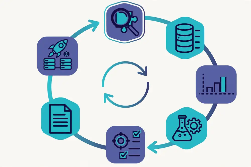
A research project is not "train a model and write it up." It is a loop with six stages: problem definition → data → baselines → experiments → evaluation → paper and deployment, and then back to problem definition, because every finished project suggests the next one. Understanding this loop changes how you work. Instead of wandering from one tutorial to another, you always know which stage you are in, what the stage's output should be, and when you are allowed to move on.

Why workflow matters more than cleverness

Beginners often believe research success comes from knowing the fanciest model. It does not. Reviewers and supervisors judge a project on four things: Is the problem clearly defined? Is the evaluation honest? Is the work reproducible? Is the writing clear? A simple logistic regression project that nails all four will beat a giant neural network project that fails them. Workflow is the machinery that produces those four qualities.

Think of the difference between coursework and research. In a course, the dataset is given, the metric is given, and the answer exists. In research, you must create all three yourself: you find or build the dataset, you choose the metric and defend it, and there is no answer key — only evidence. That is why workflow matters. Without it, you drown in decisions. With it, each decision has a place and a time.

The six stages in brief

Stage 1 — Problem definition. You state exactly what you are solving and how you will measure success. This is a written sentence, not a feeling. A good problem statement at this stage saves you weeks later, because it tells you what data to collect and which papers to read.

Stage 2 — Data. You find, collect, clean, and label data. This is usually 50–70% of a real project's effort. Students chronically underestimate it. The data stage also includes ethics: consent, privacy, and permission.

Stage 3 — Baselines. You run the simplest reasonable methods first and record their scores. Baselines are your honest starting line. Everything you do later is measured against them.

Stage 4 — Experiments. You run the loop: form a hypothesis, run the experiment, analyze the result, and decide the next step. This is where the actual research happens, and where tracking matters most.

Stage 5 — Evaluation. You measure your best model on held-out data with the right metrics, and you study its errors. This stage answers the reviewer's question: "Should I believe these numbers?"

Stage 6 — Paper and deployment. You write the work up in the standard structure, release code and data so others can reproduce it, and build a demo that makes the work real. Deployment is optional for some papers but powerful for presentations and impact.

Notice the loop: a deployed system and a written paper always reveal the next problem. The error analysis in Stage 5 hands you Stage 1 of the next project. Research is a spiral, not a line.

A realistic timeline

For an MS thesis-level project with one student working part-time, a sensible calendar looks like this: problem definition and literature review, 3–5 weeks; data collection and labeling, 4–8 weeks; baselines and experiments, 6–10 weeks; evaluation and error analysis, 2–3 weeks; writing and revision, 3–4 weeks; demo and presentation, 1–2 weeks. That is roughly one semester of real work. The biggest beginner mistake is spending 80% of the time on experiments and leaving data and writing squeezed into the final week. Protect the writing time — a brilliant result nobody can understand is not a result.

Worked example: the crop-disease classifier

Meet our running example. A master's student, let's call her Ayesha, works at a university in an agricultural region. Farmers near her campus lose tomato crops to leaf diseases every season, and the local agriculture office diagnoses diseases slowly, by sending samples to a distant lab. Ayesha's idea: build an image classifier that tells a farmer whether a tomato leaf is healthy or diseased, from a phone photo taken in the field.

Her first instinct is to download a famous public dataset of leaf photos, train a deep learning model, and report 95% accuracy. That is a coursework project, not research. When she reads the literature (Chapter 3), she discovers something interesting: published models score above 90% on clean lab photos but drop to 65–75% on real field photos with messy backgrounds, shadows, and multiple leaves. Nobody has tested these models on field photos from her region. That becomes her gap, and her project: can a classifier trained on lab photos plus a modest set of local field photos reach reliable accuracy on local field photos? The chapters ahead follow this project stage by stage — the problem statement, the literature table, the data collection, the baselines, the experiments, the evaluation, the paper, and the demo.

The researcher's mindset at each stage

Each stage has a different mental mode. In problem definition, be a skeptic: attack your own idea before reviewers do. In data, be a detective: assume the data is hiding problems until you prove otherwise. In experiments, be a scientist: change one thing at a time and write down what you expected before you see the result. In evaluation, be an auditor: try to disprove your own numbers. In writing, be a teacher: your reader was not there for the journey. Practicing these modes is what turns a student into a researcher.

Common ways projects derail (and how the workflow prevents them)

Most struggling projects fail in predictable ways, and each failure maps to a skipped stage. Tutorial hell: the student completes course after course on model architectures but never defines a problem — cured by Chapter 2's problem statement, which forces commitment. Data collected without a question: months of gathering images or scraping text, then the horrible realization that the data cannot answer any interesting question — cured by defining the problem and reading the literature first. The "one more experiment" trap: endless tuning with no stopping rule, so the paper never gets written — cured by Chapter 7's stopping rules and Chapter 1's calendar. Writing left to the final week: the results exist but cannot be communicated, and the deadline passes — cured by protecting writing time from the start and drafting figures early (Chapter 9). No version control, no tracking: the best result cannot be reproduced, so it cannot be published — cured by Chapter 6's five non-negotiables. Notice the pattern: every derailment is a stage done out of order or skipped. The workflow is not bureaucracy; it is the collected memory of thousands of failed projects, organized so you do not have to fail the same way.

There is also a subtler derailment: solving the wrong problem well. A student builds a beautiful 97%-accurate classifier for a task nobody needs, on data nobody trusts, and wonders why no venue wants it. The defense is external contact, early and often: talk to the farmer, the doctor, the engineer — whoever lives with the problem — before you commit. Ayesha spent two afternoons at the agriculture office before writing her problem statement. Those conversations gave her the diagnosis-delay fact that anchored her motivation section and the realism that kept her project honest. No tutorial teaches that; the workflow demands it.

How to use this book alongside your project

Do not read this book cover to cover and then start. Use it as a field manual. Before you begin: read Chapters 1–3 and produce a problem statement and a literature summary table. During data work: keep Chapter 4 open; do the pilot before the full collection. During experiments: live in Chapters 5–8; the experiment log template and the hypothesis template are daily tools. When results stabilize: read Chapters 9–10 and start the paper and the code release in parallel — writing will surface gaps in your experiments while there is still time to fill them. Before your presentation: Chapters 11–12. And when the project ends, return to Chapter 1: your error analysis has already written the first paragraph of your next problem statement. The loop continues.

For your research: Before you read further, write down your current project idea in one paragraph. Then answer three questions honestly: (1) What exactly would "success" look like as a number? (2) What data would you need, and do you have access to it? (3) What is the nearest published work, and what did it not do? If you cannot answer all three, your next job is not training a model — it is Chapters 2 and 3 of this book. Bring these answers to your supervisor; they will immediately respect the seriousness of your preparation.

Key takeaways - An AI research project is a loop of six stages: problem definition, data, baselines, experiments, evaluation, and paper/deployment. - Reviewers judge clarity of problem, honesty of evaluation, reproducibility, and writing — not model fanciness. - Data work usually takes more than half the project's time; plan for it. - Budget writing time from the start; do not squeeze it into the final week. - Every stage has a mental mode: skeptic, detective, scientist, auditor, teacher.

---

Chapter 2: Defining the Problem Precisely

Most failed research projects do not fail at training. They fail at the first sentence: nobody — not the student, not the supervisor, not the reviewer — can say exactly what the project is trying to do. A vague problem produces vague data, vague experiments, and a paper that reviewers reject with the dreaded phrase "unclear contribution." This chapter teaches you to write problem statements that survive review.

What a problem statement is and is not

A problem statement is a precise, written claim: what task you are solving, on what data, measured how, compared against what. It is not a topic ("AI in agriculture"), not a dream ("help farmers"), and not a method ("use deep learning"). Methods belong later; the problem statement is method-free. It says what must be achieved, not how you will achieve it.

Compare these: - Weak: "I want to use deep learning to help farmers detect plant diseases." - Strong: "Build an image classifier that labels tomato leaf photos taken in the field as healthy, early blight, or late blight, reaching at least 85% accuracy on a held-out set of photos from farms in Punjab, compared against a ResNet-50 baseline trained only on lab images."

The strong version names the input (field photos), the output (three classes), the metric (accuracy), the test condition (held-out Punjab farm photos), and the comparison (a specific baseline). A reviewer reading it knows exactly what would count as success. That is the standard you are aiming for.

The four components of a surviving problem statement

Every strong problem statement has four parts:

1. Context and motivation. Why does this matter, and to whom? One or two sentences. Cite a real fact if you can — crop losses, diagnosis delays, cost of lab testing. Motivation tells the reviewer why they should care; it does not prove anything by itself.

2. The gap. What exactly is missing in current work? This must be specific and evidence-based, not "no one has done this before" (which is usually false or means nobody cared). Good gaps: prior work used lab images but not field images; prior work did not test on your region's crop varieties; prior work compared no baselines; prior work is too heavy for a phone.

3. The objective. What you will build or test, stated without method hype. "Evaluate whether adding N field photos to training improves field-image accuracy" is an objective. "Use a novel hybrid attention transformer" is a method looking for a problem.

4. The success criterion. The number and the comparison. Name the metric (accuracy, F1, error rate), the test data, and the baseline you must beat. If you cannot name these now, you are not ready to start experiments — go back to the literature.

Making it measurable: metrics and constraints

Beginners often pick accuracy because it is familiar, then discover their classes are imbalanced and accuracy lies. If 90% of your leaves are healthy, a model that always says "healthy" scores 90% accuracy and is useless. For imbalanced problems, F1-score (the balance of precision and recall) or per-class accuracy tells the truth. Choose your metric before you run experiments, write it in the problem statement, and do not change it after seeing results — changing the metric to favor your model is a classic integrity failure that reviewers spot instantly.

Also state your constraints: the model must run on a phone, or train on a single GPU, or work with only 500 labeled images. Constraints turn a generic project into an interesting one, and they protect you from scope creep — when your supervisor suggests adding five more diseases, you can point at the written scope.

Scope control: the art of saying "not yet"

The number one killer of student projects is scope creep. "While you're at it, add the other crops. And make it real-time. And write the mobile app." Each addition sounds small and each one doubles the work. A good problem statement is a shield: it defines what is in and, by omission, what is out. Keep a "future work" list. Everything that is not in the problem statement goes there — visibly, so your supervisor agrees it is parked, not forgotten.

A useful trick: the minimum publishable unit. Ask, "What is the smallest result that would still be a real contribution?" For Ayesha, it is: a classifier for three tomato leaf classes on local field photos, honestly evaluated, compared to a baseline. The mobile app, the other crops, the real-time video — those are future work. Finish the minimum unit first. You can always expand; you cannot un-collapse a project that grew too big.

The stranger test

Before the supervisor meeting, try the stranger test: read your problem statement to someone outside your field — a friend, a family member — and ask them to restate it in their own words. If they can say what task you are doing, how you will measure success, and what you are comparing against, the statement is clear. If they say "something with AI and plants," rewrite. Researchers are blind to their own jargon; the stranger is a cheap, honest detector. Ayesha's first draft failed the stranger test ("deep learning for farmers" came back as "an app, maybe?"); her final draft passed ("you're checking whether adding local photos helps a tomato-disease photo classifier, and you need 85% on new farms to win"). Clarity for a stranger is clarity for a reviewer.

Worked example: Ayesha's problem statement, refined

Ayesha's first draft was: "Use deep learning to detect tomato diseases and help farmers." After two weeks of reading (Chapter 3), she rewrote it:

"Tomato growers in Punjab lose an estimated 20–30% of yield to foliar diseases, and lab diagnosis takes 5–7 days. Published leaf-disease classifiers reach 92–96% accuracy on lab-condition images but report 65–75% on field photos [to be filled with real citations]. No published work evaluates these models on field photos from Pakistani farms. Objective: build an image classifier for three classes (healthy, early blight, late blight) that reaches ≥85% accuracy on a held-out set of 300 field photos from 10 Punjab farms. Comparison: a ResNet-50 baseline trained only on public lab images. Constraint: inference must run on a mid-range Android phone in under 2 seconds."

Notice what this does: it justifies (losses, delay), names the gap (no evaluation on Pakistani field photos), states the objective and number, names the baseline, and sets a constraint. Her supervisor approved it in one meeting. The project now has rails.

Problem statements for different kinds of contributions

Not every paper proposes a new method, and the problem statement should reflect the kind of contribution you are making. For an application paper (Ayesha's kind), the statement emphasizes the new domain or condition: "evaluate method X on data/condition Y, where it has never been tested." For a comparison or benchmark paper, the statement emphasizes fairness: "compare the leading approaches A, B, and C on a unified benchmark with identical splits and metrics, which no prior work has done." For a methods paper, the statement emphasizes the deficiency being fixed: "existing methods fail under condition Z; we propose a modification and measure whether it closes the gap." The four components (context, gap, objective, success criterion) stay the same; what changes is where the novelty lives. Beginners often write a methods-style statement ("we propose a novel architecture") for what is really an application project — and then reviewers judge the architecture's novelty and find it thin. Match the statement to the contribution you can actually deliver. An honest application statement beats a grandiose methods statement every time.

Getting sign-off: the problem statement meeting

A problem statement is not finished when you like it; it is finished when your supervisor approves it in writing — an email, a signed page, a comment on the document. Supervisors see failure modes you cannot: the dataset you cannot access, the metric the community does not respect, the gap that was closed last year. Bring three things to that meeting: the statement itself, the one-page evidence for the gap (from your literature table), and your list of parked future-work items. Ask explicitly: "Is this the right scope? Is the metric acceptable? What would make you reject this project in month four?" The answers are a gift — they are the reviewer's objections, delivered early, when they are still cheap to address. If the evidence later forces the statement to change (it sometimes does — data may refuse to cooperate), that is fine: revise it, re-gather evidence, and get sign-off again. A problem statement is a living contract, not a prison. What it cannot be is vague — vagueness is just a deferred argument with your supervisor, and deferred arguments are always more expensive.

For your research: Write your problem statement now, in the four-part format, aiming for under 150 words. Then perform the "hostile reviewer test": imagine the toughest reviewer in your field reading it and list the three objections they would raise (vague metric? no comparison? gap not evidenced?). Rewrite to answer each objection. Repeat until you cannot find a new objection. A statement that survives your own hostility will survive review. Keep every draft — your thesis or paper's introduction will be built from the final one.

Key takeaways - A problem statement names the task, data, metric, test condition, and baseline — never just a method or a dream. - The gap must be specific and evidence-based: what did prior work not do, and why does it matter? - Choose your metric before experiments and never change it to flatter your results. - State constraints; they make the project interesting and control scope. - Define the minimum publishable unit and park everything else as future work.

---

Chapter 3: Literature Review as the Foundation

A literature review is not a chore you do to satisfy your supervisor. It is the foundation of the entire project: it tells you what has been tried, what worked, what failed, and where the empty space is. A sloppy review means you will "discover" things that were published five years ago — the fastest route to rejection. A good review, by contrast, hands you your problem statement, your baselines, your datasets, and your metrics on a plate.

Where to search and what counts

Start with Google Scholar for breadth. Then go to the venues that matter in your subfield: for AI, the big conferences (NeurIPS, ICML, ICLR, CVPR, ICCV, ECCV, ACL) and journals (IEEE Transactions, Pattern Recognition, Computers and Electronics in Agriculture for our running example). For applied work, domain journals matter as much as AI venues — an agriculture-AI paper belongs in an agriculture journal's conversation too. Your university library gives you access to IEEE Xplore, ScienceDirect, and Springer; learn to use them now, because paywalls are part of a researcher's life.

What counts as a citable source? Peer-reviewed conference and journal papers first. Then reputable preprints (arXiv) — fine to read, but prefer the peer-reviewed version when it exists. Textbooks like Russell and Norvig [1] or Goodfellow et al. [5] for background concepts. Technical reports from known labs occasionally. What does not count: blog posts, Medium articles, undocumented GitHub repos, and vendor whitepapers. You may learn from them, but do not cite them as evidence. And never cite a paper you have not at least skimmed — reviewers can tell, and mis-cited papers are embarrassing when caught.

How to read 30 papers without drowning

You do not read every paper word for word. Use the three-pass method. Pass one (5 minutes): read the title, abstract, figures, and conclusion. Decide: relevant or not? Pass two (20–30 minutes): read the introduction, method overview, key figures and tables, and results. You now understand the paper's claim and evidence. Pass three (only for the 5–8 most important papers): read everything, including details, and try to reproduce the key idea mentally. Most papers get passes one and two only. This is not laziness — it is triage, and every working researcher does it.

While reading, take notes in a fixed template for each paper: problem addressed, method used, dataset, metric and result, limitation (stated or visible), and how it relates to your project. The limitation column is the gold mine — authors often bury the most useful sentence in their "limitations" or "future work" paragraph, and that sentence is frequently your research gap wearing a disguise.

The summary table: your review's engine room

Do not write your review as a list of paragraphs ("Paper A did X. Paper B did Y."). That is a bibliography with verbs — reviewers hate it. Instead, build a summary table: rows are papers, columns are problem, method, dataset, metric, key result, limitation. Once the table exists, the patterns jump out: everyone used the same dataset; nobody tested on field images; the best-reported accuracy clusters around 93% on lab data; two papers mention field performance dropping but did not investigate it. Your literature review chapter then writes itself as a story about these patterns, ending at the gap.

Aim for 25–40 papers for a thesis-level review, 15–25 for a conference paper's related work. Quality beats quantity: ten deeply understood papers beat fifty skimmed ones. And keep the table alive — add papers as you find them during the project, because the experiments phase will surface new related work you missed.

Finding the gap: four reliable patterns

Genuine gaps usually take one of four shapes. Learn to recognize them:

1. The dataset gap. A method works on dataset A but has never been tested on dataset B, and there are reasons to expect different behavior. (Ayesha's gap: lab images vs. Pakistani field images.)
2. The condition gap. The method assumes conditions that fail in practice — clean images, balanced classes, abundant labels, powerful hardware. Your work tests or fixes the realistic condition.
3. The comparison gap. Papers each report their own numbers on their own setups, and nobody has compared the main approaches fairly on one benchmark. A careful comparison study is a legitimate contribution.
4. The deployment gap. The method is accurate but too slow, too big, or too fragile for real use. Making it practical — smaller, faster, robust — is real research, not "just engineering."

Beware the fake gap: "nobody has combined model X with dataset Y." If there is no reason to expect the combination to matter, reviewers will ask "so what?" A gap needs a why — a reason the missing piece matters to someone.

Organizing and citing as you go

Use a reference manager from day one — Zotero (free) or Mendeley. Every time you read a paper, save the PDF and the citation immediately. Nothing is more miserable than writing a paper with 30 citations assembled from memory at 2 a.m. Learn your venue's citation style early (this book uses IEEE numbered style [1], [2]) and keep a single .bib file or library for the whole project. When you write, cite claims the moment you make them; a paragraph with no citations in a related-work section is a paragraph that should not exist.

Worked example: Ayesha's review

Ayesha searched Google Scholar for "plant leaf disease classification deep learning" and "PlantVillage field images," then followed citations forward and backward from the most-cited papers. Her summary table had 28 rows. The pattern was stark: 24 papers used the PlantVillage lab dataset; 3 used other lab datasets; exactly 1 attempted field images, reporting a 20-point accuracy drop, and none used images from Pakistan. Two papers noted in their limitations that "field robustness remains untested." She had her gap, her baselines (the two most-cited CNN approaches), her metric (accuracy on held-out field images, plus F1 for the minority disease class), and her dataset plan (public lab images + self-collected field images). The review took four weeks. It saved her from at least three dead ends she would otherwise have discovered by failing.

Reading critically: evaluate, don't just collect

A summary table tells you what papers claim; critical reading tells you whether to believe them. For each important paper, ask: Was the evaluation fair? Did they compare against strong, well-tuned baselines, or strawmen? Did they test on a proper held-out set? Do the numbers support the story? Check whether the headline improvement survives the reported variation — a 1-point gain with ±2 points of noise is not a finding. Are the ablations convincing? If a paper claims component X matters but never tests the model without X, the claim is decoration. And watch for the citation telephone game: paper A reports a result with caveats, paper B cites it without the caveats, paper C cites B as established fact. When a claim matters to your project, trace it back to the original source and read the caveats yourself. Ayesha caught one of these: a widely cited "field accuracy" number turned out, in the original paper, to be accuracy on lab images with synthetic noise added — not field images at all. Her summary table flagged it, and her gap survived because she checked.

When to stop reading and start doing

Literature review has diminishing returns, and perfectionists can read forever. Use the saturation rule: when new papers stop changing your summary table's patterns — same datasets, same methods, same reported ranges, same unaddressed gap — you have read enough to start. For most student projects this happens around 25–40 papers. Stopping does not mean the review is closed: keep a "new papers" habit of one search per month during experiments, because the field moves and a competitor may publish your gap. But the review's job at the start is to authorize action, not to be exhaustive. Ayesha stopped at 28 papers when three consecutive searches added rows but no new patterns. She started collecting data the following Monday. Six weeks later, a new preprint appeared on field robustness — she read it, added a row, cited it in related work, and adjusted one baseline. That is the healthy rhythm: a solid foundation, then maintenance.

For your research: This week, build a summary table with at least 15 papers in your area, using the columns: problem, method, dataset, metric, key result, limitation. Then write one paragraph answering: "What is the pattern, and where is the gap?" Show the table and the paragraph to your supervisor before you collect a single data point. If your supervisor cannot see the gap from your table, your review is not done. Remember: every claim in your eventual paper's related-work section must trace back to a paper you actually read — never invent citations, and never cite from abstracts alone.

Key takeaways - The literature review gives you the problem, baselines, datasets, and metrics — it is the project's foundation, not a formality. - Search Google Scholar plus your subfield's real venues; cite peer-reviewed work you have actually read. - Use the three-pass reading method and a fixed note template; the limitation column is where gaps hide. - Build a summary table, then write the review as a story about patterns ending at the gap. - Real gaps come in four shapes: dataset, condition, comparison, deployment — each needs a "why it matters." - Manage references from day one with Zotero or Mendeley; never invent or pad citations.

---

Chapter 4: Data Collection, Labeling, and Ethics

If models are the engine of AI, data is the fuel — and most beginners put dirty fuel in the tank. Researchers consistently report spending half to two-thirds of project time on data: finding it, cleaning it, labeling it, and understanding it. This chapter covers how to do that work properly, including the ethics that reviewers and institutions increasingly demand.

Start with existing data — and interrogate it

Before collecting anything, exhaust existing sources. Public datasets (like PlantVillage for leaf images), government open-data portals, and datasets released with papers are free starting points. But never trust a dataset on reputation alone. Interrogate it: How was it collected? Under what conditions? Who labeled it, and how were disagreements resolved? What is the class balance? Are there near-duplicates between the supposed train and test portions? Download it, plot the class distribution, look at 50 random samples with your own eyes, and check image sizes, formats, and metadata. Ayesha did this with PlantVillage and found it clean but entirely lab-condition — white or grey backgrounds, single centered leaves. That finding shaped her whole project: the public data could train the model, but it could not test the real-world claim.

Document everything you learn in a dataset sheet: source, collection method, size, class distribution, known limitations, license, and citation. This becomes the dataset paragraph of your paper, and reviewers increasingly expect it. If the dataset has a license, respect it — "publicly downloadable" is not the same as "free to republish."

Collecting your own data: plan before you shoot

When existing data cannot answer your question, you collect your own. This is powerful — a well-built new dataset is itself a publishable contribution — but it must be planned. Write a collection protocol before you start: what exactly to capture, under what conditions, with what equipment, and how much you need. Ayesha's protocol specified: tomato leaves photographed with mid-range Android phones, in natural field light, at three times of day, across 10 farms, aiming for at least 100 photos per class, with each photo tagged by farm, date, and variety.

Two rules save enormous pain. First, collect more than you think you need — you will discard 10–30% for blur, wrong framing, or ambiguous cases. Second, record metadata at capture time: farm, date, phone model, lighting. Metadata you skip now is metadata you cannot reconstruct later, and it is exactly what error analysis (Chapter 8) will need. A simple spreadsheet filled in the field beats a perfect database designed afterward.

Labeling: where quality is decided

Labels are the ground truth your model learns from, so label quality caps model quality. For Ayesha's project, each photo needed a label: healthy, early blight, or late blight. She could not label them herself — she is not a plant pathologist — so she partnered with the university's agriculture department, and an agronomist labeled each image. That expert involvement is worth stating in your paper; it is a credibility signal reviewers notice.

Follow these labeling practices: - Write labeling guidelines first. One page with definitions and example photos for each class, including the hard cases ("yellowing from nutrient deficiency is NOT early blight"). Give it to every labeler. - Double-label a subset. Have two people independently label 10–20% of the data and measure agreement. Low agreement means your guidelines — or your class definitions — are unclear. Fix the guidelines, not the labelers. - Handle ambiguity honestly. Some photos will be genuinely uncertain. Create an "uncertain/exclude" bucket rather than forcing a guess. Forced guesses become label noise, and label noise becomes a model that confidently learns the wrong thing. - Keep the labelers blind to your hypothesis. If labelers know which photos are "supposed" to be hard, it biases them. This sounds fussy; it is standard scientific practice.

Budget realistically: expert labeling is slow and sometimes costly. Ayesha's agronomist labeled 400 photos in about 12 hours spread over two weeks. Plan this into your timeline (Chapter 1) and be grateful, professional, and prompt with your collaborators.

Splits: the line between honest and dishonest results

Split your data into train (model learns), validation (you tune hyperparameters and pick models), and test (final score, touched once). The deadly sin is leakage: information from the test set influencing training. The classic beginner version is testing on training data. The subtle version is splitting by photo instead of by farm: if photos from the same farm appear in both train and test, the model may learn farm-specific backgrounds rather than disease signs, and your test score will be a lie.

Ayesha split by farm: 6 farms for training, 2 for validation, 2 held out for testing. Her test accuracy dropped compared to a naive random split — and that lower number was the honest one. When a reviewer asks "how did you split?", "by farm, to prevent background leakage" is an answer that builds trust. Also lock the test set early and do not peek at it during development. Every peek is a small leak; enough peeks and your test set becomes a second validation set.

Ethics: consent, privacy, and permission

AI ethics is not only about giant tech companies. If your data involves people, farms, or private property, you have obligations. Ayesha needed permission from farm owners to photograph on their land, and she explained in plain language what the photos were for. If your data includes people — faces, medical images, survey responses — you likely need informed consent and possibly approval from your institution's ethics board. Start that process early; boards are slow.

Three practical rules: (1) Collect the minimum you need. Do not photograph the farmer's family because the camera was handy. (2) Anonymize. Strip names, GPS coordinates, and identifying details unless your research question requires them, and store data securely. (3) Be honest about use. If you told farmers the photos were for research, do not later sell them to a company. Your paper's ethics or data statement should describe consent and handling in two or three sentences — reviewers increasingly look for it, and its absence is noticed.

Worked example: Ayesha's dataset

Final tally: 38,000 public lab images (PlantVillage tomato subset) for training support, plus 1,240 self-collected field photos from 10 farms. After expert labeling and discarding 180 ambiguous or blurry photos, she had 1,060 usable field images: 420 healthy, 350 early blight, 290 late blight. Split by farm into train/validation/test. The agronomist double-labeled 150 photos with a second expert; agreement was 94%, and disagreements were resolved by discussion and documented. Total data effort: six weeks. It was the longest single phase of her project — and the reason her later results meant something.

Storing and versioning data practically

Data needs the same version discipline as code. At minimum, keep a data/ folder with subfolders per version (v1-pilot/, v2-full/) and a README in each describing what changed, when, and why. Never overwrite a dataset in place — the day you need to compare against last month's version, you will be glad the old one still exists. For larger projects, tools like DVC (Data Version Control) track data versions alongside git commits, so a given code commit points to the exact data it ran on. Whatever system you use, record a simple fingerprint for each version — the number of samples per class and a checksum or hash of the files — in your experiment log. Then any run's "data version" field (Chapter 6) is meaningful. And back up: keep at least two copies of irreplaceable collected data in different places (laptop plus external drive or cloud). Ayesha's field photos existed in three places from the day they were taken. Collected data is the one project asset that cannot be regenerated by re-running code — treat it as irreplaceable, because it is.

Working with domain experts: respect earns quality

When your labels or problem understanding depend on experts — agronomists, doctors, engineers — remember that you are asking busy professionals for their scarcest resource: attention. Make it easy for them: bring the labeling guideline with examples, a simple interface (even a shared folder of images with a spreadsheet beats a clunky custom tool), and a realistic estimate of the time needed. Batch questions instead of interrupting daily. Show them early results — experts who see their labels producing a working model become invested collaborators rather than reluctant helpers. Discuss authorship and acknowledgment upfront with your supervisor: a domain expert who shaped the problem and validated labels has often earned more than a thank-you line. Ayesha's agronomist ended up as a co-author, and his field knowledge improved the paper's discussion section beyond anything she could have written alone. Finally, close the loop: share the finished paper and the demo with every expert and data provider. It is professional courtesy, and it keeps the door open for your next project.

For your research: Before collecting data, write a one-page collection protocol (what, how, how much, metadata) and a one-page labeling guideline (class definitions + examples). Show both to your supervisor and, if applicable, your domain expert. Then do a pilot: collect and label 50 samples end-to-end, run them through your whole pipeline, and check that everything works. The pilot will reveal every flaw in your protocol while it is still cheap to fix. Document consent and permissions in writing — a short signed note from each data provider protects you and satisfies reviewers.

Key takeaways - Interrogate any existing dataset before trusting it: collection method, labeling, balance, leakage, license. - Plan collection with a written protocol; record metadata at capture time; collect more than you need. - Label quality caps model quality: guidelines, expert labelers, double-labeling, honest handling of ambiguity. - Split by the right unit (farm, patient, speaker — not individual samples) to prevent leakage; lock the test set. - Handle ethics properly: permission, informed consent, minimum collection, anonymization, honest use.

---

Chapter 5: Baselines First — Why Simple Models Come Before Fancy Ones

Every beginner wants to start with the most powerful model they have heard of. Resist this. The professional move — the one that separates researchers from hobbyists — is to build the simplest reasonable baseline first, measure it carefully, and only then try anything fancier. This chapter explains why, and how to choose baselines that make your eventual results meaningful.

What a baseline is and why it is non-negotiable

A baseline is a simple, well-understood method run on your problem before your "real" method. It answers the question every reviewer asks: "Is your fancy method actually better than the obvious thing?" Without a baseline, your 87% accuracy is a lonely number. With a baseline at 81%, your 87% is a six-point improvement — a claim. With a baseline at 86.5%, your 87% is noise — and you need to know that before you write the paper, not after a reviewer tells you.

Baselines also debug your pipeline. If a simple logistic regression scores 50% on a three-class problem — barely above chance — something is broken: labels, data loading, or splits. If you had started with a 50-layer network, you would blame the architecture and waste weeks tuning. The baseline tells you the pipeline works, the data is learnable, and the problem is real. Géron's hands-on guide [2] makes the same point from the practitioner's side: start simple, establish the pipeline end to end, then improve.

Choosing good baselines: the ladder

Build a small ladder of baselines, from dumb to decent:

1. Trivial baselines. Majority-class predictor ("always guess healthy") and random guessing. These cost nothing and calibrate your metric — if your model cannot beat "always guess the majority class," stop and investigate.
2. Classical machine learning. Logistic regression, random forests, or SVMs on hand-crafted features (for images: color histograms, texture features), using scikit-learn [3]. These are fast, need little data, and are surprisingly strong.
3. Published prior work, re-run. Take the best method from your literature review and run it on your data as the authors described. This is the baseline reviewers care about most: "we beat the state of the art" only means something if you actually ran the state of the art.
4. Ablated versions of your own method. Once you have your method, baselines include your method with each new piece removed (Chapter 7 covers ablations properly).

For Ayesha: trivial baseline (majority class: 40% accuracy), logistic regression on color histograms (68%), and a published ResNet-50 approach re-trained on her data (74% on field test). That ladder took two weeks. Everything afterward was measured against it.

How many baselines are enough?

A common question: is two baselines enough, or do I need ten? The answer is coverage, not count. You need enough baselines that a reviewer cannot say "but did you try the obvious thing?" For most student projects, three to five well-chosen baselines cover the space: one trivial, one classical, and one to three serious contenders (re-run prior work plus ablated versions of your method). More than that, and you are spending paper pages and compute on diminishing returns; fewer, and the comparison looks thin. One more consideration: match the baselines to your claim. If your claim is "our method is more accurate," the baselines must be accuracy-competitive. If your claim is "same accuracy but 10× faster," you need a speed comparison table too — accuracy baselines alone do not support an efficiency claim. Write your claim first (it comes from the problem statement), then check that every word of it has a baseline behind it. Unbacked adjectives are where reviewers strike. When in doubt, include the baseline and let the table speak — an extra row costs little, but a missing obvious comparison costs credibility.

The baseline trap: weak baselines that flatter you

There is a dishonest version of this chapter, and reviewers know it: the strawman baseline — an intentionally weak or badly tuned baseline that makes your method look good. Examples: comparing against a published method but training it for far fewer epochs, using default hyperparameters for the baseline while tuning yours for weeks, or evaluating the baseline on harder data. This is one of the most common reasons papers get rejected, and experienced reviewers detect it quickly.

The rule is symmetric effort: give baselines a fair, documented tuning effort. You do not need to tune them as obsessively as your method, but you must describe what you did — "baseline hyperparameters tuned via grid search on the validation set, same as our method" — so the comparison is credible. When your method barely beats a well-tuned baseline, that is still a result: report it honestly. A small honest win beats a large suspicious one.

What baselines teach you about the problem

Baselines are diagnostic instruments. Watch what they reveal: If classical ML reaches 80% of the deep model's score, your problem may not need deep learning — and "a simple model suffices" is itself a publishable finding. If all baselines fail on a specific subset (say, shaded leaves), you have found the hard core of the problem before spending a month on architecture search. If the trivial baseline scores suspiciously high, your metric or split is probably broken. Ayesha's logistic regression hitting 68% told her the color signal was strong — diseased leaves really do look different in color space — which later justified her hypothesis that color augmentation would help.

Worked example: Ayesha's baseline week

Ayesha gave herself a strict two-week baseline budget. Week one: data pipeline (loading, augmentation, splits) plus trivial and classical baselines. Week two: re-running the published ResNet-50 baseline from her literature review, following the paper's described settings, tuned lightly on her validation farms. Results on the held-out test farms: majority class 40%, logistic regression 68%, ResNet-50 74%. She wrote these numbers in her experiment log, committed the code, and froze the test set. Only then did she allow herself to think about improvements. Her supervisor's comment: "Now whatever you build, we'll know if it worked."

Baselines beyond classification

The baseline habit applies to every task type, not just classification. For regression (predicting a number, like crop yield), the trivial baselines are predicting the training mean or median for every input — your model must beat "always guess the average." The classical step is linear regression or a random forest. For ranking or retrieval, the trivial baseline is random ordering and the classical step is a simple TF-IDF or nearest-neighbor approach. For generation or forecasting, naive baselines like "repeat the last value" are famously hard to beat and deeply informative when they win. The principle never changes: start with the dumbest thing that could work, then the standard classical method, then published prior work. Whatever your task, ask: "What would a competent non-ML practitioner try first?" That is your baseline. If your sophisticated method cannot beat it, you have learned something important — either the task needs rethinking or the sophistication is misplaced.

Documenting baseline effort for the paper

Baselines do not just live in your log; they live in your paper's method section, and reviewers scrutinize them. Write one short paragraph per serious baseline covering three things: what it is (architecture or algorithm, with citation), how it was trained (data, epochs, key hyperparameters), and how it was tuned ("hyperparameters selected by grid search over {…} on the validation set, matching the tuning budget of our method"). That last clause is the anti-strawman shield — it tells the reviewer the comparison was fair. If a baseline comes from a published paper, say whether you re-ran it or quote their reported number, and if you quote, confirm the dataset and metric match yours exactly (Chapter 8 covers this trap). Ayesha's paper had a compact "Baselines" paragraph: majority-class, logistic regression on color histograms (C tuned on validation), and the published ResNet-50 re-trained with the authors' described settings plus a small learning-rate search. Three sentences each. No reviewer questioned her comparisons — the documentation answered before they could ask.

For your research: Before your next training run, implement the trivial baseline (majority class / random) and one classical baseline on your data today. If either surprises you — trivial baseline too high, classical baseline at chance — stop and debug your pipeline before touching any neural network. Write the baseline scores in a dated log entry with the exact code version. When you later write your paper, these numbers become your results table's first rows, and the story of "simple to strong" becomes one of the most convincing narratives in research writing.

Key takeaways - Always run baselines first: trivial, classical ML, and re-run published prior work. - Baselines debug your pipeline, calibrate your metric, and make your improvements measurable. - Never use strawman baselines; tune baselines fairly and document the effort. - Baselines diagnose the problem: they reveal whether deep learning is needed and where the hard cases are. - Freeze baseline scores in a dated log before improving anything.

---

Chapter 6: Experiment Tracking and Organization

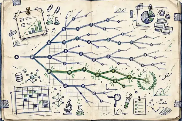
Here is a scene every researcher knows: you trained 40 models over three weeks, one of them scored brilliantly, and now you cannot remember which hyperparameters it used, which data version it trained on, or whether the score was on validation or test. That brilliant result is now worthless. Experiment tracking — the boring discipline of recording exactly what you ran and what happened — is what separates a pile of GPU hours from a research project. This chapter gives you a system.

What to track: the five non-negotiables

Every experiment run must record five things, no exceptions:

1. Code version. Which exact code ran? Use git and record the commit hash. "The script as of Tuesday" is not a version. If you tweaked the code mid-run, that is a new version.
2. Data version. Which dataset, which split, which preprocessing? If you re-labeled 50 images or changed the split, the data version changed. Keep a simple version number or hash for datasets.
3. Hyperparameters. Learning rate, batch size, epochs, architecture choices, augmentation settings, random seed — everything. These are the knobs; without them the run cannot be reproduced.
4. Environment. Library versions (PyTorch [8], scikit-learn [3], CUDA), hardware (which GPU), and the date. "It worked on my machine" dies here, documented.
5. Results. Metrics on train, validation, and test (test only at the end), plus the saved model checkpoint and a few example predictions. Also record what you expected — the hypothesis — so you can later distinguish "confirmed" from "got lucky."

Miss one of the five and the run is not reproducible. Miss it habitually and your thesis becomes archaeology.

Tools: from notebook to tracker

Start where you are. A dated lab notebook (a markdown file or actual notebook) with one entry per experiment — date, hypothesis, config, result, next step — beats a fancy tool used inconsistently. Many students run their whole thesis on a well-kept experiment log plus git. When runs multiply, graduate to a tracking tool: MLflow and Weights & Biases are the standard choices; both log hyperparameters, metrics, and artifacts with a few lines of code. TensorBoard works for metric curves. The tool matters less than the habit: every run logged, the same way, every time.

Whatever you use, adopt a naming convention and enforce it. Ayesha used YYYYMMDD-hypothesis-shortconfig, e.g., 20261103-cropfield-aug-color-lr0.001. Six months later she could read a run's name and know what it was. "final_model_v7_REAL" is not a name; it is a cry for help.

What a good log entry looks like

Abstract advice becomes concrete with an example. Here is one of Ayesha's actual-style entries:

2026-11-03 — run 20261103-cropfield-aug-color-lr0.001 Hypothesis: color-jitter augmentation will raise accuracy on shaded field photos, because baseline errors concentrate on shaded leaves (see error notes 2026-10-28). Config: configs/cropfield_aug_color.yaml (champion + color jitter p=0.5, strength 0.2); seed 42; data v2; code @a3f9c1d. Result: val accuracy 76.8% (champion 74.0%). Shaded subset: 71.2% → 77.4%. Sunny subset: 76.1% → 75.0%. Interpretation: hypothesis supported; gain concentrated where predicted. Slight sunny regression — try lower strength next. Next: 20261104-cropfield-aug-color-weak with strength 0.1.

Six lines: hypothesis, exact config reference, result with the comparison, subset breakdown, interpretation, and the next step already chosen. Anyone — Ayesha in six months, her supervisor, a reviewer — can follow the reasoning. Contrast with the entry this replaces: "tried augmentation, got 76.8%, seems good." The first is research; the second is a diary. Write the six-line version every time, and the paper's method section will assemble itself from these entries.

Organizing the project: folders that scale

A project that lives in one folder with 60 scripts named train_final2.py will collapse. Use a simple, standard layout:

project/
├── data/            # raw + processed data (or README pointing to storage)
├── notebooks/       # exploration only — never the "real" pipeline
├── src/             # the real code: data loading, models, training, evaluation
├── configs/         # one config file per experiment (YAML/JSON)
├── runs/            # outputs: logs, checkpoints, metrics — one folder per run
├── paper/           # the paper draft, figures, tables
└── README.md        # what this is, how to run it, in what order

Two principles: configs, not code edits — an experiment differs from another by its config file, not by commented-out lines in the script; and notebooks are for exploring, scripts are for running — the moment an experiment matters, it becomes a script plus a config, committed to git. Ayesha's rule: if a result might go in the paper, it must be reproducible from src/ + a config + a seed. No exceptions.

The experiment log: your project's memory

Keep a single chronological log — Ayesha used EXPERIMENTS.md — where each entry has: date, run name, hypothesis ("adding color-jitter augmentation should help shaded leaves"), config reference, validation result, and a one-line interpretation ("+2.1 points on shaded subset; hypothesis supported"). This log becomes three things later: your memory when writing the paper, your defense against reviewer questions ("why did you choose X?"), and the raw material for the ablation study. Write the interpretation before you run the next experiment; uninterpreted numbers accumulate into confusion.

Review the log weekly with your supervisor. A 15-minute walkthrough of "what I tried, what happened, what I think it means, what I'll try next" is the most productive meeting format in research. It forces you to interpret rather than just accumulate, and it catches doomed directions early.

Worked example: Ayesha's tracking setup

Ayesha's stack was deliberately simple: git for code, a configs/ folder of YAML files, MLflow for metric logging, and EXPERIMENTS.md as the narrative log. Run 20261103-cropfield-aug-color-lr0.001 tested color-jitter augmentation: validation accuracy 76.8% vs. baseline 74.0%, with the gain concentrated on shaded-leaf photos — exactly as hypothesized. Because the config, seed (42), data version, and code hash were all logged, she could re-run it bit-for-bit six weeks later when a reviewer-equivalent (her supervisor) asked. Total overhead of this discipline: maybe 10 minutes per run. Total value: her entire results section.

Tracking when you collaborate

Solo tracking is discipline; team tracking is diplomacy. When two or more people run experiments, agree on the conventions before the first run: the shared naming scheme, the shared log file or tracking server, and who owns which hypothesis thread. The classic team failure is two students unknowingly running near-identical experiments for a week, or one overwriting another's checkpoint. Prevent it with a 10-minute weekly sync where each person states their current hypothesis and next run — the meeting from Chapter 6, now with an audience. Use a shared tracking tool (MLflow and Weights & Biases both support teams) so runs are visible to everyone, and protect the main code branch: experiment in personal branches, merge through review. Ayesha's lab adopted a simple rule — no run counts unless it is logged in the shared tracker with the author's name — and inter-student duplicated work dropped to zero. The log becomes the lab's collective memory, which is exactly what a supervisor needs when writing the group's next grant.

Recovering from a messy start

If you are reading this chapter with 60 untracked scripts and a results table built from memory, do not despair — retrofit. The freeze-and-document protocol: (1) Stop and commit everything to git as-is, mess included; tag it pre-cleanup. (2) Re-run your key results — baselines and champion — from the current code with fixed seeds, logging all five non-negotiables this time. If a result does not reproduce, that is vital information: mark it unverified and re-earn it. (3) Write the README and the experiment log retroactively for the runs that matter, noting honestly which details are reconstructed. (4) Going forward, the new system applies with no exceptions. This takes a few days and feels like going backward; it is actually the moment your project becomes real. Ayesha's labmate did this in his third month and discovered his headline number had come from a validation-set evaluation mislabeled as test — caught in time, fixed, and the paper was stronger for the honest correction. A messy start is forgivable. A messy finish is not.

For your research: Today, set up the minimum viable system: a git repo, a configs/ folder, a runs/ folder, and an EXPERIMENTS.md file with your first entry (your baselines from Chapter 5). Adopt a run-naming convention and write it at the top of the log. Then make a rule and keep it: no result counts unless it is logged with code hash, data version, hyperparameters, seed, and validation metric. Show the log to your supervisor at your next meeting — it is the single clearest signal that you are running a professional project.

Key takeaways - Track five things per run: code version, data version, hyperparameters, environment, results (+ hypothesis). - Use a consistent tool (notebook log → MLflow/Weights & Biases) and a strict run-naming convention. - Organize by folders: data, notebooks (exploration only), src, configs, runs, paper, README. - Experiments differ by config file, not by edited code; important results must be re-runnable from script + config + seed. - Keep a chronological experiment log with interpretations; review it weekly with your supervisor.

---

Chapter 7: The Experimental Loop — Hypothesis, Run, Analyze, Iterate

Experiments are where research actually happens, and most students do them wrong: they change five things at once, run overnight, see a number go up, and declare victory without knowing why. The professional alternative is the experimental loop: form a hypothesis, run a controlled experiment, analyze the result, and let the analysis choose the next step. This chapter makes that loop concrete.

Start with a hypothesis, not a hyperparameter

A hypothesis is a testable prediction with a reason: "Adding color-jitter augmentation will improve accuracy on shaded field photos, because the baseline's errors concentrate on shaded leaves and color jitter simulates lighting variation." Note the structure: prediction + mechanism + evidence for the mechanism (the error analysis). "Maybe a bigger model will help" is not a hypothesis — it is a wish. Wishes produce random walks; hypotheses produce knowledge even when they fail.

Write the hypothesis in your experiment log before running. This single habit defeats the most common self-deception in research: HARKing (hypothesizing after the results are known) — seeing a number go up and inventing a story for why. Reviewers can often smell HARKed stories because the "explanation" does not quite fit the experiment. Pre-registered hypotheses keep you honest, and failed hypotheses are still findings: "color jitter did not help; errors are about occlusion, not lighting" is a publishable insight.

One variable at a time: the controlled experiment

Change one thing per experiment. If you change the architecture, the learning rate, and the augmentation simultaneously and the score improves, you have learned nothing — you cannot say which change mattered. This is the same principle as a school science fair, and researchers violate it constantly under deadline pressure.

The practical pattern: keep a champion (your current best config) and test challengers that differ by exactly one factor. Ayesha's champion was the ResNet-50 baseline at 74.0%. Challenger 1: champion + color jitter → 76.8%. Champion becomes the color-jitter version. Challenger 2: new champion + extra field photos in training → 79.5%. Each step is attributable. When she later wrote her ablation table, it practically wrote itself, because the loop had generated it.

Analyze, don't just admire, the number

A single accuracy number is the beginning of analysis, not the end. For every run, ask four questions: 1. Did it beat the champion on validation? By how much, and is the gap bigger than run-to-run noise? (Re-run with a different seed if the gap is small — a 0.3-point "improvement" that vanishes with seed 43 is noise, not progress.) 2. Where did the change help or hurt? Break results down by subset: per class, per farm, shaded vs. sunny, easy vs. hard. Ayesha's color jitter helped shaded leaves (+6 points) but slightly hurt sunny ones (−1 point) — a nuance that became a paragraph in her paper. 3. What do the errors look like now? Sample 30–50 mistakes and look at them. Error analysis (Chapter 8) is not a final stage; do a light version after every important run. 4. What does this rule out? A failed experiment eliminates a hypothesis. Record the elimination. Negative results are data.

Also watch for regression in disguise: overall accuracy up, but one class collapses. If your "improvement" sacrifices the rare disease class that matters most to farmers, it is not an improvement. Per-class metrics catch this; a single headline number hides it.

Iterate: letting results choose the next step

Iteration is a decision procedure, not vibes. After each analysis, one of four things happens: (1) Adopt — the challenger clearly wins; it becomes the champion. (2) Reject — it fails or ties; record why and move on. (3) Refine — it helps partially; form a narrower hypothesis (e.g., "color jitter helps, but the strength is too high for sunny images — try weaker jitter"). (4) Pivot — repeated failures suggest the hypothesis family is wrong; go back to error analysis and find a new direction.

Set a stopping rule before you start a line of experiments: "I will try at most 5 augmentation variants; if none beats the champion by 1 point, I move on." Without stopping rules, you will tune one idea forever. Research progress comes from breadth of ideas tested cheaply, not depth of tuning on one idea. A useful budget: no single idea gets more than a week without a clear win.

When to stop experimenting altogether

Experiments end; papers begin. Stop when: your results answer the problem statement's question (Ayesha: can we reach 85% on field photos? — yes, 86.2%); additional experiments give diminishing returns (three straight ideas fail to move the number); or your timeline says writing must start (Chapter 1's calendar is a commitment). Perfection is the enemy: a paper reporting 86% with honest analysis beats a never-finished quest for 90%. You can always run the next idea as future work — or as your next paper.

Beware the sunk-cost experiment

The hardest part of the loop is not technical — it is emotional. After three weeks tuning one idea, abandoning it feels like wasting three weeks. That feeling has a name, the sunk-cost fallacy, and it has killed more projects than bad hyperparameters. The weeks are already spent; the only question is what the next week buys. A clean kill criterion, written before you start ("five variants, need +1 point, then move on"), makes quitting a decision instead of a defeat. Ayesha killed a two-week architecture exploration that never beat the champion — and the freed month went into the field-photo experiments that actually moved the number. Remind yourself: a rejected hypothesis documented in the log is a contribution to your understanding. An idea tuned forever in hope is just expensive procrastination.

Worked example: Ayesha's loop in action

Over five weeks, Ayesha ran 23 challenger experiments. The log tells the story: color jitter (+2.8, adopted), extra field photos in training (+2.7, adopted), stronger augmentation (−1.2, rejected — over-regularized), class-weighted loss (+0.9 on the rare class, adopted for fairness), bigger architecture (+0.4, rejected — not worth the phone-deployment cost), test-time augmentation (+0.6 but 4× slower, parked as future work). Final validation: 86.2%. Every adopted step had a hypothesis written beforehand; every rejection had a reason. When her supervisor asked "why this architecture and these settings?", she opened the log and read the story. That story became her paper's method section.

Designing experiments that fail informatively

Not all failed experiments are equal. A good failed experiment discriminates between explanations: it rules something out. "I tried a bigger model and it didn't help" rules out little — maybe the model was too big, the tuning too short, the data too small. Compare: "I hypothesized errors came from lighting variation, so I added color jitter; accuracy unchanged, and errors are still concentrated on shaded leaves — therefore lighting variation is not the main cause; the next hypothesis is occlusion." The second failure is progress: it killed a hypothesis cleanly and pointed at the next one. Design for this by stating, alongside each hypothesis, what a negative result would mean. And keep a negative-results section in your log. Negative results feel like wasted time, but they are the map of explored territory — they stop you (and your labmates) from re-exploring it, and they sometimes become the most interesting part of a paper's discussion. Science advances as much by ruled-out explanations as by confirmed ones; your log should reflect that.

Balancing intuition and discipline

The loop described in this chapter sounds rigid, and beginners sometimes hear "never follow a hunch." That is not the message. Intuition — the pattern-matching your brain does after weeks immersed in data — is a genuine research asset; many breakthroughs start as "this feels like it might work." The discipline is not to suppress hunches but to route them through the loop: write the hunch as a hypothesis (forcing yourself to articulate the mechanism), test it as a single-variable challenger, and let the analysis judge it. What the loop forbids is hunch-driven conclusions — declaring victory because it felt right. Ayesha's best idea (adding field photos to training) started as a hunch over tea; it became a result because she tested it against the champion with everything else fixed. Keep a "wild ideas" list in your log for hunches that do not fit the current thread, and give yourself one time-boxed exploration slot per week — say, Friday afternoon — for undisciplined play. Structure on weekdays, play on Friday: the loop stays clean, and the hunches still get their chance.

For your research: Before your next experiment, write the hypothesis in this exact template: "I predict [change] will [effect] on [metric/subset], because [mechanism], based on [evidence from error analysis or literature]." Run the experiment changing one variable. Then write the analysis answering the four questions above before you run anything else. Do this five times and you will feel the difference: you are no longer "trying things" — you are conducting research. Bring the log entries to your supervisor; the hypotheses will make the meeting dramatically more useful.

Key takeaways - Every experiment starts with a written hypothesis: prediction + mechanism + evidence. No HARKing. - Change one variable at a time; keep a champion and test single-factor challengers. - Analyze beyond the headline number: subsets, per-class metrics, error samples, seed noise. - Iterate by decision: adopt, reject, refine, or pivot — with a stopping rule per idea. - Stop experimenting when the problem statement's question is answered or returns diminish; ship the paper.

---

Chapter 8: Evaluation and Error Analysis in Practice

This is the chapter reviewers read first — the results section — and the stage where honesty is tested. Evaluation is not "report the biggest number you saw." It is a disciplined argument that your numbers mean what you claim. Done right, it makes your paper bulletproof. Done sloppily, it is the reason most papers are rejected.

The golden rule: test once, on locked data

Your test set has been locked since Chapter 4. Now you may touch it — once, with your final model (or a small set of finalists). Report that number. If you evaluate ten models on the test set and report the best, you have turned the test set into a validation set and your number is optimistic. This is so common it has a name — test-set overfitting — and reviewers probe for it by asking how many times you evaluated on test.

In practice: do all model selection on validation. When the champion is chosen and frozen, run it on test, record the metrics, and that is your paper's headline number. Ayesha's champion scored 86.2% on validation and 84.7% on the locked test farms — a small, honest drop that actually increased trust, because a test score above validation would have smelled like leakage.

Metrics: report the right ones, all of them

Report accuracy (readers expect it), per-class precision, recall, and F1 (the truth about imbalanced classes), and a confusion matrix (which classes get confused with which). For Ayesha: overall 84.7% accuracy, but the confusion matrix showed early blight confused with late blight in 12% of cases — the two diseases look similar in early stages. That single matrix did more work than any paragraph: it showed she understood her model's real behavior.

Add confidence intervals or seed variation: train your final model with 3 different seeds and report mean ± standard deviation. "84.7% ± 0.9%" tells a reviewer the result is stable; a bare "84.7%" invites the question "or did you get lucky?" If your improvement over the baseline (74.0%) is 10 points with ±0.9% noise, the win is real. If it were 0.5 points, it would be noise — report that honestly too.

Fair comparison: the results table

Your results table is the heart of the paper. Every row is a method (baselines first, then yours), every column a metric, all evaluated on the same test set with the same metric. Include the trivial and classical baselines from Chapter 5 — their presence signals honesty. Ayesha's table: majority class 40.0%, logistic regression 68.2%, published ResNet-50 74.0%, hers 84.7%. The story reads itself: each step contributed, and the gap to prior work is large enough to matter.

Never compare your test number against a baseline's validation number, or your tuned model against an untuned baseline (Chapter 5's symmetric-effort rule). And never report only the metric where you win while hiding the one where you lose — if your method is slower or bigger, say so. Reviewers reward candor; they punish selective reporting.

Error analysis: turning failures into findings

Error analysis is the systematic study of what your model gets wrong, and it is the most underused tool in student research. Procedure: take 50–100 test errors, look at each one, and categorize: What kind of image? What kind of mistake? Ayesha found three patterns: (1) shaded leaves misclassified as diseased (model confusing shadow for lesions), (2) early-stage infections missed (genuinely hard — even the agronomist hesitated), (3) multiple leaves in frame confusing the classifier.

Each pattern becomes something valuable: pattern 1 suggests a preprocessing or augmentation fix (future work); pattern 2 sets realistic expectations and justifies the "early detection is hard" discussion; pattern 3 becomes a deployment note ("photograph a single leaf"). Two of these went into her paper's discussion section; one became her next project's problem statement. Your errors are your next paper's introduction. Also report the flip side: check 30 correct predictions to make sure the model is right for the right reasons, not exploiting a spurious cue (like a farm's distinctive soil color in the background).

Report the cost, not just the score

Modern reviewers increasingly ask: what did this result cost? Report training time and hardware for your final model and key baselines — "trained in 6 hours on a single RTX 3060" — so readers can judge practicality. If your method needs 10× the compute of the baseline for a 1-point gain, say so; the trade-off is part of the finding, and hiding it invites suspicion. For the paper, a single sentence in the method section plus a column in the results table (training hours, inference milliseconds per image, model size in MB) is enough. Ayesha's table had an inference-time column, which is also what let her defend the phone-deployment constraint in Q&A later. Cost reporting is honest, it is increasingly expected, and it often reveals that the "best" model is not the most useful one — which is itself a result worth discussing.

Statistical sanity and honest language

You do not need advanced statistics, but you need honest language. Say "outperformed the baseline by 10.7 points on the test set" — not "proved superior" or "state of the art" (unless you truly compared against all credible contenders). Say "suggests" when the evidence is suggestive. Never write "our model solves" — models do not solve; they score. And acknowledge threats to validity: small test set, single region, one phone model. A short "limitations" paragraph does not weaken your paper; it preempts the reviewer's objections and shows maturity. Ayesha's limitations: 300 test images from 2 farms, one crop, one season. Honest, specific, and each one a future-work arrow.

Worked example: Ayesha's evaluation

Final protocol: champion model (ResNet-50 + color jitter + field photos + class-weighted loss), trained with 3 seeds, evaluated once on the locked 300-image test set from 2 unseen farms. Results: 84.7% ± 0.9% accuracy; per-class F1: healthy 0.91, early blight 0.79, late blight 0.83. Baseline comparison table as above. Confusion matrix showed the early/late blight confusion. Error analysis of 60 mistakes yielded the three patterns. She wrote the results section in two days because the experiment log already contained everything — the numbers, the comparisons, the error categories. Evaluation felt like assembly, not invention, because the discipline had been built in Chapters 5–7.

Comparing against published numbers without re-running

Sometimes you cannot re-run prior work — the code is unavailable, the compute is prohibitive, or the paper predates code-release norms. Then you may quote their reported numbers, but under strict conditions. First, verify the comparison is apples-to-apples: same dataset, same split protocol, same metric. Papers often evaluate on different test splits of "the same" dataset, and those numbers are not comparable — say so explicitly if that is the case. Second, label quoted numbers as quoted: a table footnote like "† reported in [5]; not re-run" is honest and standard. Third, prefer re-running the one or two most important competitors even if you quote the rest; a paper whose central claim rests entirely on quoted numbers is fragile. Ayesha re-ran the top-cited ResNet-50 baseline but quoted two older SVM-based results with daggers, noting the split difference. A reviewer asked about one quoted number; her footnote answered it before the question was finished. The rule: quote transparently or re-run — never silently mix your fresh numbers with someone else's reported ones as if they came from the same experiment.

Qualitative evaluation: showing, not just scoring

Numbers convince reviewers; pictures convince everyone else — and they often reveal what numbers hide. Build a small qualitative figure: 6–12 example inputs with your model's predictions, including both successes and instructive failures. For Ayesha: three correctly classified leaves, one shaded-leaf error, one early-infection miss, each with the model's confidence. This figure does triple duty: it makes the paper readable, it demonstrates you have looked at your model's behavior (reviewers notice), and it becomes your best presentation slide. You can also run a tiny human comparison: have your domain expert classify 50 test images and report human accuracy alongside the model's. If the model matches the expert on easy cases but trails on hard ones, that is a meaningful, honest characterization of where the technology stands. One caution: choose qualitative examples representatively, not as a highlight reel. A figure of only perfect predictions is advertising; a figure with failures analyzed is research.

For your research: Right now, write down your evaluation protocol before you need it: (1) What is your locked test set, and when was it locked? (2) Which metrics will you report? (3) Which baselines go in the comparison table? (4) How many seeds will you run? Tape this to your wall. When evaluation day comes, follow it exactly — the temptation to "just try one more model on test" will be strong, and this note is your defense. Then do a 50-error analysis on your current best model this week; categorize the errors and bring the categories to your supervisor. That one exercise will improve your project more than a week of tuning.

Key takeaways - Touch the locked test set once, with the frozen final model; all selection happens on validation. - Report accuracy plus per-class precision/recall/F1, a confusion matrix, and seed variation (mean ± std). - Build a fair comparison table: same test set, same metrics, honest baselines, symmetric tuning effort. - Do systematic error analysis (50–100 errors, categorized); errors become discussion points and future work. - Use honest language ("outperformed by X points"), acknowledge limitations, never overclaim.

---

Chapter 9: Writing the Paper — IEEE Conference Structure Section by Section

Good research badly written is unpublished research. Writing is not the final chore; it is the moment your work becomes real to the world. This chapter walks through the standard IEEE conference paper structure — the format most CS/AI venues use — section by section, with practical advice for each. The structure is a contract with your reader: they know where to look for everything, so your job is to put the right thing in each place.

Before you write: assemble your materials

Writing goes fast when the materials exist. Gather: your problem statement (Chapter 2), your literature summary table (Chapter 3), your dataset sheet (Chapter 4), your experiment log with the champion's config (Chapters 6–7), your evaluation numbers and error analysis (Chapter 8), and your figures. Then write the figures and tables first — the results table, the confusion matrix, the method diagram, the error examples. A paper is an argument built around its figures; if the figures tell the story, the text just narrates it. Ayesha laid out five figures on her desk before writing a word.

Get the IEEE template early (IEEE Conference template, two-column) and write in it from the start. Formatting at the end is painful; writing in the template keeps you honest about the page limit (usually 6–8 pages plus references) and forces concision.

Title and abstract: the 200 words that decide everything

Most people who encounter your paper will read only the title and abstract. The title should name the task and the contribution: "Field-Robust Tomato Leaf Disease Classification by Combining Lab and Field Images" — specific, searchable, honest. Avoid cute titles, avoid "novel," avoid "using deep learning" (everyone uses deep learning).

The abstract (150–250 words) has a fixed job in four moves: (1) the problem and why it matters (2–3 sentences); (2) the gap in prior work (1–2 sentences); (3) what you did and the key result with numbers (3–4 sentences); (4) the implication (1 sentence). Write it last, even though it appears first. Every claim in the abstract must appear with evidence in the body — reviewers check this.

Introduction: the funnel

The introduction is a funnel: wide at the top (the problem domain and its importance), narrowing to the gap (what prior work missed, with citations), narrowing to your contribution (what you did, listed explicitly). End with a contribution list — 3–4 bulleted claims: "We collected a field-image dataset of 1,060 labeled photos from 10 farms; we show that adding field photos to training raises field accuracy from 74.0% to 84.7%; we analyze error patterns and release code and data." Reviewers read the contribution list and then check whether the paper delivers each item. Make sure it does — every bullet must be evidenced in the results.

Related work: the story, not the list

This is your literature review (Chapter 3) compressed into 1–1.5 pages. Organize by theme, not by paper: "Lab-image disease classifiers," "Field-robustness studies," "Lightweight models for mobile deployment." Within each theme, describe what the group achieved and where it falls short, citing as you go. End each theme — and the section — pointing at your gap. The classic beginner failure is the laundry list ("[3] did X. [4] did Y."); the fix is synthesis: compare, contrast, and conclude. Every paragraph should end with the reader understanding why your work was needed.

Method: reproducibility on paper

Describe what you did precisely enough that a competent reader could reimplement it: dataset (size, splits, collection — cite your dataset sheet), model architecture, training procedure (optimizer, learning rate, epochs, augmentation, seeds), and evaluation protocol (metrics, validation vs. test). Include the details beginners omit: input image size, normalization, class weighting, hardware, library versions [8]. If space is tight, put extended details in an appendix or the code release — but the paper alone should let a reader understand every number in your results table. When in doubt, imagine a skeptical reviewer asking "how exactly did you get 84.7%?" and answer them here.

Results: show, then tell

Present the comparison table first — it is the paper's centerpiece. Then walk the reader through it: the baselines, your method, the ablations (each component's contribution, from your Chapter 7 log). Use the confusion matrix and error-analysis figures. Report numbers with their variation (± std over seeds). Describe, don't hype: "Adding field photos improved test accuracy from 74.0% to 79.5%" — the numbers speak. Save interpretation for the discussion: what the error patterns mean, why the method works, where it fails. This is also where limitations live — a short, honest paragraph (Chapter 8).

Conclusion and references

The conclusion restates the problem, the key result, and the implication in half a page — no new claims, no new numbers. End with 2–3 concrete future-work directions (the parked ideas from Chapter 2's scope control). Then the references: every citation real, every entry accurate, formatted in IEEE numbered style [1]–[8]. Check each one: does the cited paper actually say what you claim? Mis-citations are easy to make and embarrassing to be caught in. Ayesha verified all 24 of hers against her summary table in one careful pass.

Revision: the paper is rewritten, not written

First drafts are supposed to be bad. Then revise in passes: pass 1 — structure (does the argument flow? does each section do its job?); pass 2 — clarity (read it aloud; cut every sentence that does not earn its place); pass 3 — precision (numbers consistent everywhere, claims match evidence, citations correct). Then get feedback: your supervisor, a senior student, anyone who will be brutal. Give them specific questions ("is the contribution clear? does the method section let you reproduce it?") rather than "what do you think?" Budget two full weeks for writing and revision — the calendar from Chapter 1 protects this time.

Worked example: Ayesha's paper

Ayesha's 6-page paper: title naming task + contribution; 180-word abstract with the 74.0%→84.7% headline; introduction funneling from crop losses to the field-robustness gap; related work in three themes; method with full training details and the by-farm split; results table with baselines, ablations, confusion matrix, and error analysis; honest limitations; conclusion with two future directions. Her supervisor's first comment: "I can see exactly what you did and why it matters." Submitted to a regional IEEE conference. The writing took three weeks — because the previous eight chapters had already done the thinking.

The most common writing mistakes (and their fixes)

Reviewers see the same writing failures repeatedly. Learn them now and your paper will stand out for its clarity. Burying the contribution: the reader reaches page 4 unsure what is new — fix with the contribution list at the end of the introduction. Inconsistent numbers: the abstract says 85%, the table says 84.7%, the conclusion says "about 86%" — fix by defining each number once and searching the draft for every mention before submitting. Undefined terms and unexplained notation: every symbol in an equation must be defined where it appears; every acronym spelled out on first use. Figure-text mismatch: the text says "Figure 3 shows X" but the figure shows Y, or figures are referenced out of order — fix by checking every figure reference in a dedicated pass. Overclaiming: "state of the art," "solves," "novel" without evidence — fix with Chapter 8's honest language. Related work as a list: fixed by Chapter 3's thematic synthesis. Missing limitations: reviewers will supply them, unkindly — fix by writing your own limitations paragraph first. Ayesha's pre-submission checklist was exactly this list, checked line by line with her supervisor. It caught two inconsistent numbers and one overclaim ("first ever" — softened to "to our knowledge, the first evaluation on Pakistani field images," which was both true and defensible).

After submission: the rebuttal

Most conferences have a rebuttal phase: reviewers ask questions, you get limited space (often one page) to respond. The rebuttal is not a second paper — it is a focused, courteous argument. Thank the reviewers sincerely; they donated their time. Answer every point, numbered, in order — even the ones you disagree with. For each: acknowledge, answer with evidence (a number, a figure, a citation), and state what you changed in the paper. Concede gracefully where the reviewer is right: "The reviewer is correct that our test set is small; we have added this as an explicit limitation and propose expanded collection as future work" — this sentence has saved many papers. Never be defensive or dismissive; the reviewer is not your enemy but a proxy for your future readers. If a requested experiment is impossible in the time allowed, say so honestly and offer what you can do (an analysis, a clarification, a smaller experiment). Ayesha's rebuttal answered 11 reviewer points in one page: 8 with new analyses from her existing log, 2 with text clarifications, 1 with an honest concession. The paper was accepted. Her log — the boring discipline of Chapters 6 and 7 — was the reason she could answer 8 points without running a single new experiment.

For your research: This week, do two things: (1) download the IEEE conference template for your target venue and read its formatting rules (page limit, reference style, figure requirements); (2) draft your paper's figures and tables now — even with preliminary numbers — as placeholders. You will discover immediately which results you are missing and which story your data wants to tell. Then write the contribution list (3–4 bullets) and pin it above your desk; every experiment from now on must serve one of those bullets, or it does not belong in the paper.

Key takeaways - Assemble materials first; build figures and tables before writing text; write in the IEEE template from day one. - Title names task + contribution; abstract does four moves (problem, gap, method + numbers, implication) in 150–250 words. - Introduction funnels to an explicit contribution list; every bullet must be evidenced in the body. - Related work synthesizes by theme and ends at your gap — never a laundry list. - Method must enable reproduction; results show honestly with variation; discussion interprets; limitations are a strength. - Revise in passes (structure → clarity → precision), get brutal feedback, and protect two weeks for writing.

---

Chapter 10: Reproducibility — Code Release, Seeds, Documentation

A result nobody can reproduce is a rumor. Reproducibility — the ability of another person to rerun your work and get the same results — has moved from a nice ideal to a hard requirement: many conferences now have reproducibility checklists, artifact evaluation, and code-submission expectations. More importantly, reproducibility protects you: six months from now, you will be the "other person" trying to rerun your own work. This chapter makes your project reproducible by construction.

The three pillars: code, data, environment

Reproducibility rests on three pillars, and all three must be shared or documented:

1. Code. The complete pipeline: data loading and preprocessing, model definition, training, evaluation. Not just the final training script — everything from raw data to results table. If a step was done by hand in a notebook, convert it to a script or document it exactly.
2. Data. The dataset (or precise instructions to obtain it), the splits, and the preprocessing. If you cannot release data (privacy, permission limits), release the split indices, the preprocessing code, and a small sample — and say clearly why the full data is restricted.
3. Environment. Library versions, Python version, OS, hardware. A requirements.txt or conda environment file with pinned versions (torch==2.1.0, not torch) is the minimum. "It worked with whatever was installed" is not documentation.

Ayesha's release checklist: GitHub repo with src/, configs/, the champion config, requirements.txt with pinned versions, a README with run commands, the trained model weights, and the field dataset with the collection protocol. Total preparation time: three days. It felt like overhead; it was actually the final quality check — she found and fixed two undocumented preprocessing steps while writing the README.

Seeds and determinism: taming randomness

Deep learning is full of randomness: weight initialization, data shuffling, augmentation, dropout. Without fixed seeds, two runs of the "same" experiment give different numbers, and your 84.7% becomes unreproducible. Set seeds for every randomness source — Python's random, NumPy, and PyTorch [8] — at the start of every script, and log the seed with the run (Chapter 6). Ayesha used seed 42 for development and seeds 42/43/44 for the final reported numbers.

Be honest about limits: exact bit-for-bit reproducibility across different GPUs is sometimes impossible (certain GPU operations are nondeterministic). What you promise is practical reproducibility: same code + same data + same seed + same library versions → same results within small noise. State your seeds in the paper's method section; reviewers increasingly look for them.

Documentation: the README test

Your repository's README is the entry point. It must let a stranger go from zero to your results table. The README test: give the repo to a labmate who has never seen it and watch them try to run it. Every point of confusion is a documentation bug. A good README has: what the project does (one paragraph), setup (environment creation, data download), the exact commands to reproduce the main result (copy-pasteable), expected outputs and runtime, and the project layout. Ayesha's README reproduced her headline number with three commands. Her labmate found one missing step (downloading the public lab images) — fixed in ten minutes, caught before any reviewer could trip on it.

Also document decisions, not just commands: why this architecture, why these splits, why this metric. A short DECISIONS.md or well-written commit messages preserve the reasoning that the code cannot show. Your future self, writing the thesis discussion section, will thank you.

Versioning and archiving: making it permanent

GitHub is for development; archiving is for permanence. When the paper is submitted, create a release (a tagged version, e.g., v1.0-paper) and archive it on Zenodo, which issues a DOI — a permanent, citable identifier. Cite the code and dataset in your paper with their DOIs. This matters because links rot: personal webpages vanish, but a Zenodo DOI persists. Many venues now expect this, and funders increasingly require it.

Keep the repo clean before release: remove dead code, API keys, absolute paths (/home/ayesha/... breaks on every other machine — use relative paths), and giant files that should be downloads instead. Run the README test one final time on a fresh machine or container. If it works there, it will work for a reviewer.

Licensing: tell people what they may do

Code and data without a license are legally unusable — "all rights reserved" by default, which means nobody can build on your work without asking. Add a LICENSE file to your repo. For code, the MIT license (permissive, simple) is the standard student choice; use GPL only if you understand its share-alike obligations. For datasets, Creative Commons licenses fit: CC-BY (use with attribution) is the common choice for research data. Match the license to your consents — if farmers agreed to research use only, say so in the dataset README and choose terms that reflect it; a license cannot grant rights you do not have. Also check your institution's policy: some universities claim IP in student work or require a specific license. One email to your supervisor or tech-transfer office now prevents an awkward takedown later. Ayesha used MIT for code and CC-BY for the field dataset, with a note that farm identities were withheld by design. Licensing takes an hour; it is the difference between "published" and "actually reusable."

Worked example: Ayesha's release

Ayesha's repo, tomato-field-disease, tagged v1.0-paper and archived on Zenodo: src/ with data/model/train/evaluate modules, configs/champion.yaml (seed 42 documented), requirements.txt pinned, model weights (85 MB), field dataset (1,060 images + labels + collection protocol + consent notes), README with three-command reproduction, and a DECISIONS.md summarizing key choices from her experiment log. Her paper cited the code and data DOIs in a "Code and Data Availability" paragraph. When a conference reviewer later asked for the per-farm split details, she answered with a link instead of a scramble.

Reproducibility starts on day one (not at submission)

Everything in this chapter is ten times harder if attempted the week before the deadline. The researchers with the cleanest releases are not more disciplined at the end — they were slightly disciplined every day. The daily habits that make release week trivial: commit code every day you work; never leave an experiment unlogged overnight; keep the README's setup instructions current as your environment changes (not "I'll document it later"); pin dependency versions the day you add them. Think of it as the new-laptop test: at any point in the project, you should be able to hand your repo to a labmate's fresh machine and have the main pipeline run. Ayesha ran this test monthly — it took 20 minutes each time and caught environment drift twice (a library update that silently changed augmentation behavior). By submission week, her "release preparation" was a single afternoon: tag, archive, write the availability paragraph. Reproducibility is not a final phase; it is a property your project has or does not have, built one habit at a time.

A note on what you cannot share

Sometimes full sharing is impossible: medical data under privacy law, industry data under NDA, or code built on a proprietary library. This does not exempt you from reproducibility — it changes its form. Share everything you legally can: the code, the preprocessing, the model architecture, the hyperparameters, synthetic or sample data that demonstrates the pipeline, and precise instructions for obtaining the restricted data (who to contact, what agreement is needed). Document exactly what is restricted and why, in both the repo and the paper. Reviewers understand genuine restrictions; what they do not accept is vagueness used as a shield. And where possible, validate on a public proxy: Ayesha could not have shared her field photos if farmers had refused consent — her fallback plan was to validate the method on a public field-image dataset from another region and release that pipeline fully. Plan the fallback before you need it, and get consent terms in writing during collection (Chapter 4) so "can I share this?" is answered before it becomes urgent.

For your research: Do the README test this month, even before your project is finished: ask a labmate to clone your repo and run your baseline from the README alone. Fix everything they trip on. Then set up this habit going forward: every Friday, check that the week's runs are reproducible from committed code + configs + seeds — a 15-minute check that prevents months of archaeology later. When you submit your paper, tag the release, archive on Zenodo, and cite the DOI. Reproducibility is not extra credit; it is part of the contribution.

Key takeaways - Reproducibility needs three pillars: complete code, data (or exact access instructions), and a pinned environment. - Fix and log seeds for all randomness sources; report them in the paper; promise practical, not bit-perfect, reproducibility. - The README must take a stranger from zero to your results table; test it on a labmate. - Document decisions, not just commands; use relative paths; remove secrets and dead code before release. - Tag a release on paper submission, archive on Zenodo for a DOI, and cite code/data in the paper.

---

Chapter 11: Deployment Basics — From Notebook to a Working Demo

Training a model in a notebook is the beginning of usefulness, not the end. Deployment means making the model usable outside your laptop: a demo page, a simple app, or a service that real users can touch. For a researcher, deployment is not about becoming a software company — it is about proof. A working demo convinces supervisors, reviewers, and audiences that your work is real in a way tables never can. This chapter covers the minimum you need.

What "deployment" means for a student project

Forget everything about cloud infrastructure and scaling. For your purposes, deployment means: someone who is not you can give your model an input and get an output, without your help. That is the bar. A simple web page where a user uploads a leaf photo and gets "early blight, 87% confidence" clears it. A phone app also clears it, but costs ten times the effort — choose the web page first.

The pipeline has four steps: (1) Export the trained model (save weights plus the exact preprocessing); (2) Wrap it in a small program that loads the model, preprocesses input, runs inference, and formats the output; (3) Serve it behind a simple interface (a web page with an upload button); (4) Test it with inputs you did not prepare — ideally with a real user in the room. Ayesha used a minimal Python web setup: one script loading her champion weights, one page for upload and results. Built in four days.

Choosing the demo stack: boring wins

You do not need to learn web development to deploy a demo. The rule is: use the most boring tool that works. For a Python ML project, that usually means Gradio or Streamlit: a dozen lines of Python gives you an upload button, a predict button, and a results display — no HTML, no JavaScript, no frontend framework. Ayesha's first demo was a Gradio interface in 15 lines; it took an afternoon. Only if the demo must run on a phone or offline would you graduate to something heavier (a mobile framework or an exported ONNX model). Resist the temptation to build a "real app" — every week spent on app polish is a week not spent on the paper, and reviewers evaluate the research, not the UI. The demo's job is to make the model touchable. Boring tools do that job fastest, and fastest is what a student timeline needs.

The unglamorous work: preprocessing parity and latency

Two deployment bugs eat every beginner. First, preprocessing parity: the demo must preprocess inputs exactly as training did — same image size, same normalization, same color handling. A model trained on normalized 224×224 images fed raw phone photos will produce confident garbage. The fix is structural: use the same preprocessing function in training and deployment, imported from the same file — never reimplement it.

Second, latency and size: a demo that takes 30 seconds per photo feels broken. Measure inference time on the actual target device (Ayesha's mid-range Android constraint from Chapter 2). If it is too slow, standard fixes exist: smaller input size, a lighter model variant, or quantization — and note that your Chapter 7 experiments already rejected the bigger architecture partly for this reason. Deployment constraints feeding back into modeling decisions is the workflow loop working as designed.

Handling the demo's edge cases honestly

Real inputs are messier than test sets. Your demo should handle: wrong input types ("that's a photo of a cat, not a leaf"), low-quality images (blurry, dark), and low-confidence predictions. For each, decide the behavior before someone discovers it live: reject non-leaf images with a clear message, warn on low quality, and show the confidence score so users can judge. Ayesha added a simple brightness/blur check with a "photo too dark, please retake" message — a 20-line addition that saved her demo twice.

Also decide what the demo does not do: it does not diagnose with certainty, it does not replace the agronomist, it does not store user photos (privacy — Chapter 4). A one-line disclaimer on the page ("experimental research demo, not a medical/agricultural advice tool") is both honest and protective.

From demo to evidence: what deployment gives your research

A deployment is not just a showpiece; it generates research value. It validates robustness: if the demo works on strangers' photos in bad lighting, your field-robustness claim is stronger than any table. It surfaces new errors: Ayesha's first public demo misclassified a variegated ornamental leaf — a failure mode her test set never contained, now logged as future work. And it creates impact evidence: usage logs, farmer feedback, photos of the demo in use — all legitimate material for your paper's discussion, your thesis, and your presentation. Reviewers and examiners love seeing that the work left the lab.

Keep the demo maintained but bounded: it needs to work for your presentation and paper review period, not forever. Note its limits in the README (works best on tomato leaves, daylight photos). A demo that honestly states its limits impresses more than one that pretends to generality.

Worked example: Ayesha's demo day

Two weeks before her seminar, Ayesha built the demo: upload page, champion model, same preprocessing module as training, confidence display, blur/darkness checks, disclaimer line. She tested it on 20 fresh photos from a farm not in any split — 17 correct, 2 uncertain-but-flagged, 1 wrong (the variegated leaf). She wrote those numbers down: they became her presentation's most persuasive slide ("live test on unseen farm: 17/20"). On seminar day, an audience member uploaded a photo from their own phone. It worked. The room's reaction did more for her project's credibility than any accuracy table.

Monitoring a deployed demo: what happens after launch

Deployment is not "finish and forget" — models meet reality, and reality changes. Set up basic monitoring from day one: log every prediction the demo makes (input metadata, predicted class, confidence, timestamp) — with user consent and without storing personal data unnecessarily. Review the logs weekly. You are watching for three things: distribution shift (inputs changing — a new phone model, a different season's lighting — silently degrading accuracy), confident errors (high-confidence wrong predictions, the most dangerous kind), and usage patterns (which classes get queried most, where users hesitate). Ayesha's logs showed a spike in low-confidence predictions during a dusty week — airborne dust was coating leaves, a condition in no training set. That observation became a dataset-augmentation idea and, later, a paragraph in her thesis. Monitoring also tells you when to retrain: when performance on recent logged inputs drops below your paper's numbers, the model is stale. For a student demo, monitoring can be a simple spreadsheet reviewed weekly; the habit matters more than the tooling. A deployed model you never look at is a rumor you once published.

When deployment itself is the contribution

For most student papers, deployment is supporting evidence. But in some venues — applied journals, systems conferences, domain conferences like agricultural informatics — the deployed system is the contribution, and the paper is judged on it. Then the problem statement changes (Chapter 2): success is measured by usability, latency, robustness in the field, or adoption — not just accuracy. The evaluation changes too: user studies, field trials, latency benchmarks, and failure-mode documentation carry the weight that ablation tables carry in methods papers. If your work heads this way, say so early to your supervisor, because the timeline and the writing both shift: you need user feedback cycles (slow) and the paper reads more like an engineering report than a science paper. Ayesha's conference paper was a science paper with a demo; her follow-up journal submission to an agriculture venue led with the deployment — farmer feedback, field-trial results, the dusty-week story. Same project, two contributions, two framings. The workflow supports both; the choice belongs in the problem statement, made deliberately.

For your research: Scope your deployment this week: define the one input, one output, and one user your demo serves, and the device it must run on. Then build the thinnest possible version — upload in, prediction out — reusing your training preprocessing module directly. Test it on 10 inputs you did not prepare and record what happens; those results are research data. Prepare a fallback: a 60-second screen recording of the demo working, for the day the Wi-Fi dies. A demo with a fallback video is professional; a demo with no fallback is a gamble.

Key takeaways - Deployment for researchers means: a stranger can give input and get output without your help. A simple web page clears the bar. - Reuse the exact training preprocessing in deployment — never reimplement it. Measure latency on the real target device. - Handle edge cases before users find them: wrong inputs, bad quality, low confidence, plus an honest disclaimer. - Deployment validates robustness, surfaces new errors, and creates impact evidence for papers and presentations. - Keep the demo bounded and maintained for the review/presentation period; always have a fallback video.

---

Chapter 12: Presenting Your Work — Slides, Demos, and Handling Q&A

You have done the work, written the paper, and built the demo. Now you must do the final, most human part: stand up and make other people understand and believe it. A good presentation does not just report results — it transfers conviction. This chapter covers slides, the live demo, and the Q&A, where presentations are won or lost.

Structure: the story arc of a research talk

A research talk is a story with four acts, and it mirrors your paper: (1) The problem — why it matters, in one slide with a concrete image (Ayesha: a diseased tomato field). Make the audience care before you make them think. (2) The gap — what prior work missed, in one or two slides. This creates the tension: something is unsolved. (3) Your approach and results — what you did and the key numbers, in three to five slides. One idea per slide; the results table gets its own slide, large enough to read from the back row. (4) What it means — error analysis insights, limitations, the demo, future work. End looking forward, not backward.

Aim for ~10 slides and ~20 minutes, with nothing smaller than 30-point font — fewer, bigger slides beat dense ones every time. And never read your slides: the audience reads faster than you speak. Slides are visual anchors; the story comes from you.

Slides that work: figures first, words last

Each slide should pass the glance test: its point must be clear in three seconds. That means: one message per slide, a descriptive title that states the message ("Field photos break lab-trained models" — not "Results"), large figures, and minimal text. Your confusion matrix, your comparison table, your error examples — these are your best slides. Tables must be readable: 4–5 rows maximum on a slide; if your paper's table is bigger, show the key rows and say the rest is in the paper.

Prepare a backup slide deck of 3–5 extra slides for anticipated hard questions: the ablation details, the per-farm breakdown, the training curves. You will not show them unless asked — but having them ready turns a scary question into a confident moment ("Great question — I have that right here").

The live demo: choreography, not improvisation

A live demo is the highest-risk, highest-reward five minutes of your talk. Choreograph it: know exactly which photo you will upload first (one you have tested), what you will say while it processes, and what the expected output is. Narrate the input honestly ("a photo taken yesterday at Farm 7, which was never in our training data"). Then — and this is the power move — invite the audience: "Anyone want to try their own photo?" An audience volunteer's photo working live is worth ten slides.

But never improvise without a net: have the 60-second fallback video ready, test the demo 30 minutes before the talk, and know your recovery line ("Let me show you the recorded run — exactly what you'd see"). Audiences forgive gracefully handled failures; they do not forgive panic.

Handling Q&A: the skill that builds reputations

Q&A is where examiners and reviewers form their final judgment of you, not just the work. The core skill is honest, direct answering:

• Listen fully, then answer. Do not start answering halfway through the question. Repeat it briefly to confirm ("You're asking whether this works on other crops?").
• Answer the question asked. The most common failure is answering a different, easier question. If you do not know, say so: "We haven't tested that — it's in our future work." Honesty about limits (Chapter 8) earns more respect than bluffing, and bluffing gets caught.
• Bridge to your strengths. "We didn't test other crops, but on the three tomato classes our per-class F1 was..." — acknowledge, then add what you do know.
• Handle the hostile question calmly. "Isn't this just applying ResNet to leaves?" Answer: "The contribution isn't the architecture — it's showing that field robustness requires field data, which no prior work had tested. The baseline comparison in our table shows the gap." Know your one-sentence contribution defense before you walk in.
• Thank the questioner when a question reveals a real weakness — examiners remember grace under pressure.

Prepare for the five questions you will always get: Why this method? Why this dataset? How does it compare to [famous paper]? What are the limitations? What is next? Write your answers down beforehand — not to memorize, but to have thought.

Worked example: Ayesha's seminar

Ayesha's 20-minute seminar: one problem slide (the field), one gap slide (lab vs. field accuracy drop), three method slides (dataset, approach diagram, training setup), two results slides (comparison table, confusion matrix + error examples), one demo (live upload, then an audience volunteer's photo), one limitations-and-future-work slide. In Q&A she handled the predictable questions with prepared answers — the bigger-model question, the two-farm limitation, the other-crops question — and left with two collaboration offers and a clear next project. The work was good; the presentation made it land.

For your research: Before your next presentation, write your one-sentence contribution defense and your answers to the five always-asked questions. Build your slide deck around the four-act story, with the results table as the centerpiece slide. Rehearse the demo twice with fresh inputs and prepare the fallback video. Then rehearse Q&A with a labmate playing the hostile reviewer — the questions that sting in rehearsal are the ones that won't sting on stage. A presentation is not a performance of perfection; it is a demonstration of clear thinking, and clear thinking is exactly what this book's workflow trains.

Key takeaways - Structure the talk as a four-act story: problem, gap, approach + results, meaning and future. - One message per slide, message-stating titles, large figures, readable tables; keep 3–5 backup slides for hard questions. - Choreograph the demo: tested first input, narrated unseen-data story, audience volunteer, fallback video ready. - In Q&A: listen fully, answer the question asked, admit what you don't know, bridge to strengths, stay calm under hostility. - Prepare the five always-asked questions and your one-sentence contribution defense in advance.

---

References

[1] S. Russell and P. Norvig, Artificial Intelligence: A Modern Approach, 4th ed. Hoboken, NJ, USA: Pearson, 2020. [2] A. Géron, Hands-On Machine Learning with Scikit-Learn, Keras, and TensorFlow, 2nd ed. Sebastopol, CA, USA: O'Reilly Media, 2019. [3] F. Pedregosa et al., "Scikit-learn: Machine learning in Python," J. Mach. Learn. Res., vol. 12, pp. 2825–2830, 2011. [4] T. M. Mitchell, Machine Learning. New York, NY, USA: McGraw-Hill, 1997. [5] I. Goodfellow, Y. Bengio, and A. Courville, Deep Learning. Cambridge, MA, USA: MIT Press, 2016. [6] F. Chollet, Deep Learning with Python, 2nd ed. Shelter Island, NY, USA: Manning, 2021. [7] Y. LeCun, Y. Bengio, and G. Hinton, "Deep learning," Nature, vol. 521, no. 7553, pp. 436–444, May 2015. [8] A. Paszke et al., "PyTorch: An imperative style, high-performance deep learning library," in Proc. Adv. Neural Inf. Process. Syst., vol. 32, 2019.

---

Glossary

• Baseline — A simple, well-understood method run first on a problem, serving as the reference point that new methods must beat.
• Checkpoint — A saved copy of a model's weights at a point during or after training, used to resume, evaluate, or deploy the best version.
• Class imbalance — A dataset condition where some classes have far fewer examples than others, making accuracy misleading and F1-score more informative.
• Confusion matrix — A table showing, for each true class, how many examples were predicted as each class; reveals which classes the model confuses.
• Cross-validation — An evaluation technique that rotates data through training and testing roles (e.g., 5-fold) to estimate performance more robustly on small datasets.
• Data leakage — Information from the test set (or future data) accidentally influencing training, producing inflated, dishonest results.
• Deployment — Making a trained model usable outside the lab, e.g., as a demo web page, app, or service.
• Error analysis — The systematic study of a model's mistakes, categorized by type, used to understand weaknesses and guide next steps.
• Experiment tracking — Recording every run's code version, data version, hyperparameters, environment, and results so work is comparable and reproducible.
• F1-score — The harmonic mean of precision and recall; a balanced metric preferred over accuracy when classes are imbalanced.
• HARKing — Hypothesizing after the results are known: inventing an explanation for a result after seeing it, instead of predicting beforehand.
• Hyperparameter — A setting chosen before training (learning rate, batch size, epochs) rather than learned from data.
• Inference — Using a trained model to make predictions on new inputs.
• Overfitting — Learning training-data noise instead of the real pattern; high training scores but poor performance on new data.
• Problem statement — A precise written definition of the task, data, metric, test condition, and baseline for a project.
• Reproducibility — The ability of another person to rerun a project and obtain the same results, via shared code, data, seeds, and environment.
• Research gap — A specific, evidence-based absence in prior work (dataset, condition, comparison, or deployment) that justifies a new study.
• Seed — The number initializing random processes; fixing it makes experiments repeatable.
• Strawman baseline — An intentionally weak or under-tuned baseline used to make a new method look better; a common cause of rejection.
• Test set — Data locked away during development and used once at the end for the final, honest evaluation.
• Validation set — Data used during development for tuning hyperparameters and selecting models; separate from the test set.
• Ablation study — Experiments that remove one component of a method at a time to measure each component's contribution.

---

Practice Exercises

1. Write a one-paragraph description of your current (or planned) project idea. Then answer: what would success look like as a single number? If you cannot answer, list the three things you must find out first.
2. Take your project idea and rewrite it as a four-part problem statement (context, gap, objective, success criterion) in under 150 words. Perform the "hostile reviewer test" and revise twice.
3. Find 10 papers related to your topic on Google Scholar. Build a summary table with columns: problem, method, dataset, metric, key result, limitation. Identify one candidate research gap.
4. Download a public dataset in your area. Interrogate it: plot the class distribution, inspect 50 random samples, check the license, and write a half-page dataset sheet noting three limitations.
5. Write a one-page data collection protocol and a one-page labeling guideline for a dataset you might build. Then run a 20-sample pilot and list everything the pilot revealed as broken.
6. Implement a trivial baseline (majority class) and one classical baseline (e.g., logistic regression with scikit-learn [3]) on your data. Record the scores with code version and seed in a dated log entry.
7. Set up your experiment tracking minimum: a git repo, configs/ and runs/ folders, and an EXPERIMENTS.md file. Log your baselines from Exercise 6 using a strict run-naming convention.
8. Write a hypothesis using the template from Chapter 7, run a single-variable challenger experiment against your champion, and write the four-question analysis before running anything else. Repeat three times.
9. Lock a test set (split by the right unit to prevent leakage). Evaluate your champion once, report accuracy, per-class F1, a confusion matrix, and seed variation — then categorize 50 errors into patterns and write one paragraph per pattern.
10. Draft your paper's figures and tables with current numbers, write the 3–4 bullet contribution list, and outline the full IEEE paper section by section. Then do the README test: have a labmate reproduce your baseline from your README alone, and fix every confusion they hit.

---

End of Book 9. Next: Book 10 — Common AI Mistakes Beginners Make.