SQL for Data Analysis

Book 22 of 50 — AstolixGen Learning Series For researcher and publication students

---

About This Book

Most research lives in tables. Your survey responses are a table. Your sensor readings are a table. Your experiment results are a table. Before you can analyze any of them — in Python, in SPSS, in a paper — you have to get the right rows and the right summaries out of the data store. That is what SQL is for.

SQL (Structured Query Language) is the universal language of structured data. It was invented in the 1970s, it is used by every major database on Earth, and unlike most technology from the 1970s, it has not been replaced — it has only grown more important. If your research touches a database, a spreadsheet bigger than Excel can handle, an electronic health record system, a sensor network, an institutional research repository, or a public dataset portal, SQL is the skill that lets you ask precise questions and get exact answers.

This book teaches SQL specifically for data analysis, not for database administration. You will not be setting up servers or tuning performance indexes (though you will learn what they are). Instead you will learn to read data with surgical precision: filter, sort, group, join, and summarize — the five verbs of almost every analysis query you will ever write.

Every chapter follows the same shape:

• Deep explanation of the concept in plain language
• Real SQL examples you can run, with sample tables and expected results
• Common errors and fixes — the mistakes every beginner makes, so you can recognize them fast
• For your research — a box connecting the chapter to publication-quality work
• Key takeaways — the essentials to remember

A single running example ties the whole book together: the Karachi Wellness Study, a fictional-but-realistic research dataset about a 12-week health intervention trial. The same four tables appear in every chapter, growing more meaningful as your skills grow. By the end, you will write queries that answer questions like a real paper's results section — "Did the exercise group lose more weight than the control group? By how much? Is the difference statistically suggestive?" — and you will know how to document every query so another researcher can reproduce your numbers exactly.

You do not need prior programming experience. You need a computer, a free database (Chapter 2 shows you the five-minute setup), and the patience to run every example yourself. Type them by hand. Reading SQL is passive; writing SQL is the skill.

How to use this book

Chapters 1–2 build your foundation and your practice database — do them in order, at the keyboard. Chapters 3–7 are the daily toolkit (reading, filtering, sorting, summarizing, grouping); each ends with a "For your research" box showing where the technique lands in a paper. Chapters 8–10 are the power tools (joins, subqueries, windows) — the chapters that separate someone who "knows some SQL" from someone who can answer any data question. Chapters 11–12 cover changing data safely and the reproducibility practices that make your work defensible.

Suggested pace: one chapter per sitting, running every query yourself against the Karachi Wellness Study database. Do the exercises as you go — especially Exercises 9 and 10, which build the documented-query habit on your own data. If you're preparing for a specific analysis, the Learning Dashboard at the end is your quick-reference: clause order, join comparison, function lookup, and query recipes on two pages. Keep this book open beside you during your first real project; by the second, you won't need it.

---

Learning Objectives

By the end of this book, you will be able to:

1. Explain what a relational database is — tables, rows, columns, keys, and relationships — and why researchers use databases instead of spreadsheets for serious analysis.
2. Install a free SQL environment and create your own database with realistic research tables.
3. Write SELECT queries that retrieve exactly the columns and rows you need, with clear aliases.
4. Filter data with WHERE using comparison operators, AND/OR/NOT, LIKE, IN, BETWEEN, and correct NULL handling.
5. Sort with ORDER BY, remove duplicates with DISTINCT, and cap results with LIMIT for exploration.
6. Summarize data with aggregate functions (COUNT, SUM, AVG, MIN, MAX) and explain how aggregates handle missing values.
7. Group data with GROUP BY and filter groups with HAVING — including the famous WHERE-vs-HAVING distinction.
8. Combine tables with all five JOIN types (INNER, LEFT, RIGHT, FULL OUTER, SELF) and diagnose join problems.
9. Write subqueries and Common Table Expressions (WITH clauses) to break hard problems into readable steps.
10. Use window functions (ROW_NUMBER, RANK, LAG/LEAD, running totals) for analysis that aggregates cannot express — rankings, before/after comparisons, cumulative trends.

---

The Running Example: The Karachi Wellness Study

Almost every example in this book uses one small dataset so you can focus on the SQL instead of learning new data each time. Here is the study design (fictional, but modeled on real intervention trials):

• Participants enroll in a 12-week wellness program and are assigned to one of three groups: control, diet, or exercise.
• Measurements (blood pressure, weight, daily steps) are taken at up to 4 visits: week 0 (baseline), week 4, week 8, week 12.
• Surveys (satisfaction scores 1–10) are collected at the end.

Four tables hold everything:

Table	Purpose
participants	Who is in the study: ID, name, age, gender, city, enrollment date
treatment_groups	The three study arms: ID, group name, intervention description
assignments	Which participant is in which group (many-to-one)
measurements	One row per participant per visit: vitals, weight, steps

Chapter 2 shows you exactly how to create and fill these tables. Every later chapter reuses them.

---

Chapter 1: Databases and SQL — The Big Picture

Why databases exist

A spreadsheet holds data. So why do researchers need databases? The answer is three words: size, sharing, and safety.

• Size. A survey with 50,000 respondents and 200 columns will make Excel crawl. A database answers a question about those 50,000 rows in a fraction of a second, without loading everything into memory.
• Sharing. Five researchers editing one spreadsheet is chaos. A database lets hundreds of users read and write simultaneously, and it resolves conflicts for them.
• Safety. Spreadsheets have no memory of "who changed what, when." A database enforces rules — this column must always be a date; this ID must be unique; you cannot delete a participant who still has measurements — and it can roll back a mistake.

The relational database is the dominant design: data lives in tables (also called relations). A table is a grid: each row (record) is one observation, each column (field) is one attribute of that observation.

participants
+--------+------------+-----+--------+------------+-----------------+
| part_id| name       | age | gender | city       | enrolled        |
+--------+------------+-----+--------+------------+-----------------+
| P001   | Ayesha R.  | 34  | F      | Karachi    | 2026-01-12      |
| P002   | Bilal K.   | 41  | M      | Karachi    | 2026-01-15      |
| P003   | Chen W.    | 29  | F      | Lahore     | 2026-01-19      |
+--------+------------+-----+--------+------------+-----------------+

That is the entire mental model. A database is a collection of tables; SQL is the language you use to ask tables questions.

Tables, keys, and relationships

Three terms carry the whole relational idea:

• Primary key. The column (or columns) that uniquely identifies each row. In participants, part_id is the primary key: no two participants share one, and it is never empty. A primary key is how the database tells Ayesha R. apart from another Ayesha R.
• Foreign key. A column that points to the primary key of another table. In assignments, the column part_id is a foreign key pointing at participants(part_id). It is the glue between tables.
• Relationship. A foreign key creates a relationship. One participant has many measurements (one-to-many). One group has many participants (one-to-many). Participants and surveys can relate through the participant ID.

Why should a data analyst care? Because almost every analysis joins tables along these key relationships. If you understand which key points to which table, you can combine any tables correctly — Chapter 8 is entirely about this.

Where SQL sits in the data world

You will hear several database names. For analysis, this is what matters:

• PostgreSQL — free, open-source, the research world's favorite. Excellent for analysis, supports every feature in this book.
• MySQL — free, open-source, the web's favorite. Very close to PostgreSQL for basic analysis.
• SQLite — free, tiny, lives inside a single file. No server to install. Perfect for learning and for small research datasets.
• SQL Server, Oracle — commercial, common in hospitals, universities, and government. Same core language, slightly different dialect details.
• BigQuery, Snowflake, Redshift — cloud "data warehouses" for very large data. Same SQL with extras.

Dialects differ in details, not in ideas. About 90% of the SQL in this book runs unchanged in all of them. Where dialects differ (date functions, string functions, limiting rows), this book shows the PostgreSQL/MySQL/SQLite versions side by side and flags the difference. For a researcher, that coverage is enough.

SQL vs. spreadsheets vs. Python vs. SPSS

A fair question: if you already know Excel or Python, why learn SQL?

• SQL vs. Excel. Excel is interactive and visual, but it cannot reliably handle millions of rows, it has no real query language, and every analysis is a sequence of manual clicks that cannot be reproduced exactly. SQL queries are text: you save them, rerun them, and share them. Reproducibility — the heart of research — is where SQL wins outright.
• SQL vs. Python (pandas). Python is more flexible and does statistics SQL cannot. But the data usually starts in a database. Pulling 10 million rows into Python to compute one average is slow and wasteful; computing the average inside the database with SQL and pulling back one number is instant. Professional workflow: SQL gets the data, Python analyzes it.
• SQL vs. SPSS/Stata. Statistical packages are excellent at modeling. They are poor at data extraction and joining. SQL is the extraction layer; the statistics package is the modeling layer.

The honest summary: SQL is the front door to research data. Even if your final analysis happens elsewhere, the query that produces the analysis dataset is SQL.

What SQL can and cannot do

SQL is a declarative language: you describe what you want, not how to compute it. SELECT AVG(weight) FROM measurements says "give me the average weight" — the database decides how to scan the table. This is different from Python, where you write the steps. Declarative code is shorter, and the database can optimize it far better than hand-written loops.

What SQL does brilliantly: filtering, joining, grouping, summarizing, ordering, and transforming tabular data.

What SQL does poorly: complex statistics (regression, hypothesis tests), machine learning, plotting, and anything iterative. For those, hand the query results to Python, R, or SPSS.

How a query travels: from text to answer

When you press Enter on a query, four stages happen inside the database:

1. Parsing. The database checks your syntax and turns the text into a structured plan ("scan measurements, filter visit_no = 0, compute average of weight_kg").
2. Optimization. The query optimizer rewrites that plan into the fastest equivalent version — choosing which table to read first in a join, whether to use an index, how to order operations. This is the payoff of declarative SQL: you describe what, and a very sophisticated program figures out the best how. A hand-written Python loop cannot do this.
3. Execution. The engine carries out the plan, reading data pages from disk or memory.
4. Return. Results stream back as a table.

Why should an analyst know this? Two reasons. First, it explains why two queries that "say the same thing" can run at wildly different speeds — the optimizer can only optimize what you expressed clearly (e.g., a sargable WHERE enrolled >= '2026-02-01' beats WHERE strftime('%m', enrolled) = '02' because the first can use an index). Second, it tells you where to look when a query is slow: the database can show you the plan (EXPLAIN in PostgreSQL/MySQL/SQLite — try EXPLAIN SELECT ... sometime and marvel).

Thinking in sets, not loops

The hardest mental shift from spreadsheets or Python is this: SQL operates on whole sets of rows at once. There are no loops, no "for each row, do…". Compare:

• Spreadsheet mindset: "go down the weight column; if the value dropped from the cell above, mark it."
• SQL mindset: "the set of rows where weight is less than the previous visit's weight" (Chapter 10's LAG).

Beginners sometimes try to force row-by-row thinking with cursors (a SQL feature that loops). Resist it. If you find yourself wanting a loop, there is almost always a set-based formulation — a join, a window function, or a grouped aggregate — that is shorter, faster, and clearer. When you catch yourself thinking "for each participant…", translate it to "for the set of participants, partitioned by…" and you are thinking in SQL.

The SQL standard and its dialects

SQL is standardized (ISO/IEC 9075), evolving from SQL-86 to SQL:2023. The standard defines the core you are learning: SELECT, WHERE, GROUP BY, JOIN, subqueries, window functions. Vendors then add extensions: PostgreSQL's RETURNING, MySQL's LIMIT, SQL Server's TOP, SQLite's pragmas.

Practical consequences for a researcher:

• Learn the standard core first — this book teaches exactly that. It transfers everywhere.
• Isolate dialect-specific bits (date functions, string concatenation, row limiting) in one place in your queries, with comments, so porting is mechanical.
• Never rely on undocumented behavior. If MySQL's lenient GROUP BY "works" on your laptop, it is still wrong — write standard SQL and it works on every system your collaborators use.

Data warehouses and lakes: where big research data lives

Beyond traditional databases, you'll meet two more terms. A data warehouse (BigQuery, Snowflake, Redshift) stores huge, cleaned, historical datasets optimized for analytical queries — think national health registries or multi-year sensor archives. A data lake stores raw files (CSV, JSON, images) cheaply at massive scale. The modern pattern — the lakehouse — queries lake files with SQL directly. For you as an analyst, the practical point is encouraging: the interface is still SQL. Whether the data sits in a SQLite file on your laptop or a petabyte-scale warehouse, Chapters 3–10 apply unchanged; only connection details and a few function names differ.

Common errors and fixes

Error	What happened	Fix
relation "Participants" does not exist	Table names are usually case-sensitive in some databases; you created participants but queried Participants	Match the exact case used at creation; prefer lowercase names always
column "weight" does not exist	Column name misspelled or from the wrong table	Check the table definition (\d tablename in PostgreSQL, DESCRIBE in MySQL)
Thinking in "rows" when the answer is a table	Beginners expect SQL to "print" one value; every query returns a table (even a 1×1 table)	Accept the table mindset: SELECT always returns rows and columns

For your research

Your Methods section will eventually say something like "data were extracted from the institutional database using SQL." Reviewers increasingly ask how the extraction was done. A researcher who can say "here is the exact query, and here is the schema it ran against" is already ahead of one who says "we downloaded the Excel file." Treat every query in this book as a future Methods paragraph.

Key takeaways

• A relational database is a set of tables linked by keys; a primary key uniquely identifies rows, a foreign key links tables.
• SQL is declarative: you state what you want, the database figures out how.
• SQL is the extraction and summarization layer; Python/R/SPSS are the modeling layer.
• Dialect differences (PostgreSQL, MySQL, SQLite) are minor for analysis work.

---

Chapter 2: Setting Up — Your First Database and Sample Tables

Choosing your environment

For this book, use SQLite if you want zero setup, or PostgreSQL if you want the industry-standard research tool. Both are free.

Option A — SQLite (5 minutes, no install on most systems):

SQLite is often already on your machine. Open a terminal and type:

sqlite3 wellness.db

That creates a file called wellness.db and opens the SQLite prompt. Every command below runs there. When you are done, the database is that single file — email it to a collaborator and they have your whole database.

Option B — PostgreSQL (30 minutes, worth it):

1. Download PostgreSQL from postgresql.org and install it.
2. Open the psql terminal and create a database: sql CREATE DATABASE wellness; \c wellness
3. Paste all the commands below.

Option C — DB Browser for SQLite (visual, beginner-friendly):

Install "DB Browser for SQLite" (free, Windows/Mac/Linux). It gives you a point-and-click window over a SQLite file, plus a tab where you type SQL. Many students learn fastest this way.

Whichever you choose, the SQL in this book is the same. Pick one and stay with it until you finish the book.

Data types: the columns' rules

When you create a table, every column gets a data type — the kind of value it may hold. The five you will use constantly:

Type	Holds	Example	Notes
INTEGER	Whole numbers	41	Ages, counts, IDs
REAL / DECIMAL	Numbers with decimals	72.5	Use DECIMAL(5,2) for money/measurements in PostgreSQL
TEXT / VARCHAR(n)	Text	'Karachi'	VARCHAR(50) limits length; TEXT is unlimited
DATE	Calendar dates	'2026-01-12'	Always write as 'YYYY-MM-DD'
BOOLEAN	True/false	TRUE	Not supported in old MySQL versions (use TINYINT)

Two special values to know early: NULL means "no value / unknown" — it is not zero and not an empty string. Chapter 4 is devoted to its traps. And PRIMARY KEY on a column means unique and never NULL.

Creating the study tables

Here is the full schema for our running example. Run each CREATE TABLE in your database now — you will use these tables for the rest of the book.

-- 1. The three study arms
CREATE TABLE treatment_groups (
    group_id   INTEGER PRIMARY KEY,
    group_name TEXT NOT NULL,
    intervention TEXT
);

-- 2. Who is in the study
CREATE TABLE participants (
    part_id    TEXT PRIMARY KEY,
    full_name  TEXT NOT NULL,
    age        INTEGER CHECK (age > 0 AND age < 120),
    gender     TEXT CHECK (gender IN ('F', 'M')),
    city       TEXT,
    enrolled   DATE
);

-- 3. Which participant is in which group (many-to-one)
CREATE TABLE assignments (
    part_id  TEXT PRIMARY KEY REFERENCES participants(part_id),
    group_id INTEGER REFERENCES treatment_groups(group_id)
);

-- 4. Repeated measurements: one row per participant per visit
CREATE TABLE measurements (
    measure_id INTEGER PRIMARY KEY,
    part_id    TEXT REFERENCES participants(part_id),
    visit_no   INTEGER CHECK (visit_no BETWEEN 0 AND 3),
    visit_date DATE,
    systolic   INTEGER,
    diastolic  INTEGER,
    weight_kg  REAL,
    steps      INTEGER
);

Read the foreign keys: assignments.part_id → participants.part_id; measurements.part_id → participants.part_id. The REFERENCES keyword tells the database "this column must match a real primary key over there" — try inserting a measurement for participant P999 and the database will refuse. That is referential integrity, and it is the reason databases beat spreadsheets for research data: impossible data cannot be entered.

Loading the sample data

Now insert the study data. (Twelve participants, three groups, measurements at up to four visits.)

INSERT INTO treatment_groups VALUES
  (1, 'control',  'General health advice only'),
  (2, 'diet',     'Calorie-controlled meal plan'),
  (3, 'exercise', 'Supervised exercise 3x per week');

INSERT INTO participants VALUES
  ('P001','Ayesha Rahman',34,'F','Karachi','2026-01-12'),
  ('P002','Bilal Khan',41,'M','Karachi','2026-01-15'),
  ('P003','Chen Wei',29,'F','Lahore','2026-01-19'),
  ('P004','Danish Ali',52,'M','Karachi','2026-01-20'),
  ('P005','Elena Petrova',38,'F','Islamabad','2026-01-22'),
  ('P006','Faisal Ahmed',45,'M','Lahore','2026-01-25'),
  ('P007','Gul Naz',31,'F','Karachi','2026-01-27'),
  ('P008','Hassan Raza',47,'M','Islamabad','2026-02-01'),
  ('P009','Iqra Sheikh',26,'F','Karachi','2026-02-03'),
  ('P010','Junaid Tariq',55,'M','Lahore','2026-02-05'),
  ('P011','Kiran Malik',36,'F','Karachi','2026-02-08'),
  ('P012','Liam Osei',43,'M','Islamabad','2026-02-10');

INSERT INTO assignments VALUES
  ('P001',1),('P002',1),('P003',1),('P004',1),
  ('P005',2),('P006',2),('P007',2),('P008',2),
  ('P009',3),('P010',3),('P011',3),('P012',3);

The measurements table is the largest — baseline plus three follow-ups. A few participants missed visits (realistic!), and a few readings are missing (NULL):

INSERT INTO measurements
  (part_id, visit_no, visit_date, systolic, diastolic, weight_kg, steps) VALUES
  -- P001 (control)
  ('P001',0,'2026-01-12',132,84,78.5,4200),
  ('P001',1,'2026-02-09',130,82,78.0,4500),
  ('P001',2,'2026-03-09',131,83,77.8,4300),
  ('P001',3,'2026-04-06',129,81,77.5,4600),
  -- P002 (control)
  ('P002',0,'2026-01-15',145,92,91.0,2800),
  ('P002',1,'2026-02-12',144,90,90.5,3000),
  ('P002',3,'2026-04-09',143,89,90.0,3100),   -- missed visit 2
  -- P003 (control)
  ('P003',0,'2026-01-19',118,76,62.0,8000),
  ('P003',1,'2026-02-16',117,75,61.8,8200),
  ('P003',2,'2026-03-16',118,76,61.5,8100),
  ('P003',3,'2026-04-13',116,74,61.2,8400),
  -- P004 (control)
  ('P004',0,'2026-01-20',150,95,88.0,2200),
  ('P004',2,'2026-03-17',148,93,87.0,2500),   -- missed visits 1 and 3
  -- P005 (diet)
  ('P005',0,'2026-01-22',138,86,85.0,3500),
  ('P005',1,'2026-02-19',135,84,83.2,3800),
  ('P005',2,'2026-03-19',133,83,81.5,4000),
  ('P005',3,'2026-04-16',131,82,80.0,4200),
  -- P006 (diet)
  ('P006',0,'2026-01-25',142,90,95.0,2600),
  ('P006',1,'2026-02-22',140,88,93.0,2900),
  ('P006',2,'2026-03-22',139,87,91.5,NULL),   -- steps not recorded
  ('P006',3,'2026-04-19',137,86,90.0,3200),
  -- P007 (diet)
  ('P007',0,'2026-01-27',125,80,70.0,5500),
  ('P007',1,'2026-02-24',124,79,68.5,6000),
  ('P007',3,'2026-04-21',122,78,67.0,6500),   -- missed visit 2
  -- P008 (diet)
  ('P008',0,'2026-02-01',136,88,82.0,4000),
  ('P008',1,'2026-03-01',134,86,80.8,4300),
  ('P008',2,'2026-03-29',133,85,79.5,4500),
  ('P008',3,'2026-04-26',132,84,78.0,4700),
  -- P009 (exercise)
  ('P009',0,'2026-02-03',128,82,68.0,6000),
  ('P009',1,'2026-03-03',126,80,66.8,7500),
  ('P009',2,'2026-03-31',124,79,65.5,8200),
  ('P009',3,'2026-04-28',123,78,64.0,9000),
  -- P010 (exercise)
  ('P010',0,'2026-02-05',152,96,98.0,1800),
  ('P010',1,'2026-03-05',149,94,96.0,3500),
  ('P010',2,'2026-04-02',147,92,94.5,5000),
  ('P010',3,'2026-04-30',145,90,93.0,6200),
  -- P011 (exercise)
  ('P011',0,'2026-02-08',131,85,74.0,4800),
  ('P011',1,'2026-03-08',129,83,72.5,6800),
  ('P011',2,'2026-04-05',128,82,71.0,7300),
  ('P011',3,'2026-05-03',126,81,69.5,7800),
  -- P012 (exercise)
  ('P012',0,'2026-02-10',140,89,86.0,3200),
  ('P012',1,'2026-03-10',138,87,84.5,5200),
  ('P012',2,'2026-04-07',136,86,83.0,6100),
  ('P012',3,'2026-05-05',135,85,81.5,6800);

That is 12 participants and 44 measurement rows. Verify it loaded:

SELECT COUNT(*) AS participants FROM participants;
-- Expected: 12

SELECT COUNT(*) AS measurements FROM measurements;
-- Expected: 44

SELECT COUNT(*) counts rows — you will use it constantly as a sanity check. Any time you load or transform data, count before and after. If the count surprises you (expect 12 participants and 44 measurements here), stop and investigate before continuing.

Your first SELECT

Try reading the data back:

SELECT * FROM participants;

* means "all columns." It returns all 12 rows. Never use SELECT * in a final analysis query (Chapter 3 explains why), but it is perfect for exploring.

Constraints deep dive: rules that protect your science

Chapter 2 used PRIMARY KEY, REFERENCES, and CHECK briefly. Here is the full defensive toolkit — every one of these is a data-quality rule the database enforces so your analysis never has to doubt the input:

CREATE TABLE survey_responses (
    response_id INTEGER PRIMARY KEY,
    part_id     TEXT NOT NULL REFERENCES participants(part_id),
    question_no INTEGER NOT NULL,
    score       INTEGER NOT NULL CHECK (score BETWEEN 1 AND 10),
    comments    TEXT DEFAULT 'no comment',
    UNIQUE (part_id, question_no)   -- one response per participant per question
);

• NOT NULL — the column must always have a value. Use it for anything your analysis requires (IDs, group assignments, primary outcomes).
• UNIQUE — no duplicates. The composite UNIQUE (part_id, question_no) prevents double-entry of the same survey — a classic fieldwork error.
• DEFAULT — fills a value when none is given. DEFAULT CURRENT_DATE timestamps every insert automatically.
• CHECK — arbitrary rules: CHECK (systolic > diastolic) encodes a physiological fact; impossible data is rejected at entry.

Design principle: push every rule you can state into the schema. Each constraint is one fewer data-cleaning step, one fewer footnote in your paper ("three impossible values were excluded"), and one fewer way for a collaborator's spreadsheet edit to corrupt the dataset.

REAL vs NUMERIC: numbers you can trust

REAL (floating point) is approximate: 0.1 + 0.2 may give 0.30000000000000004. For sensor readings and weights this is harmless — the noise dwarfs the error. But for anything counted or financial (doses, payments, sample counts), use exact types: INTEGER for counts, DECIMAL/NUMERIC for exact decimals (PostgreSQL, MySQL). Rule: measurements → REAL, money/counts → INTEGER or DECIMAL. And never compare REALs for exact equality (WHERE weight_kg = 78.5 may miss due to representation); compare with a tolerance or round first.

Loading real data: CSV imports

Real projects don't hand-type INSERTs. Each database has a bulk loader:

-- SQLite (in the sqlite3 shell):
-- .mode csv
-- .import measurements.csv measurements

-- PostgreSQL:
-- COPY measurements(part_id, visit_no, visit_date, systolic, diastolic, weight_kg, steps)
-- FROM '/data/measurements.csv' WITH (FORMAT csv, HEADER true);

-- MySQL:
-- LOAD DATA INFILE '/data/measurements.csv'
-- INTO TABLE measurements FIELDS TERMINATED BY ',' IGNORE 1 LINES;

Workflow that prevents disasters: import into a staging table first (measurements_raw), run Chapter 5's exploration queries against it (counts, ranges, distinct values), then INSERT INTO measurements SELECT ... FROM measurements_raw with cleaning. The raw file stays untouched — your audit trail from field to database.

Inspecting your database

Forgot a column name? Every database can describe itself:

-- PostgreSQL:  \d measurements        (in psql)
-- MySQL:       DESCRIBE measurements;
-- SQLite:      .schema measurements    (in the shell)
-- Standard SQL (all three):
SELECT column_name, data_type
FROM information_schema.columns
WHERE table_name = 'measurements';

information_schema is part of the SQL standard — a set of read-only views describing the database itself. "What tables exist? What columns does each have?" is always one query away.

Natural vs surrogate keys: choosing primary keys

Our study uses part_id values like 'P001' — a natural key (meaningful to humans). The alternative is a surrogate key: a meaningless auto-generated number (1, 2, 3…). Which should you use?

	Natural key ('P001')	Surrogate key (1, 2, 3…)
Readable in query results	✅ 'P009' tells you it's a participant	❌ 9 could be anything
Stable over time	⚠️ numbering schemes change	✅ never changes meaning
Safe to expose	⚠️ may encode info (enrollment order)	✅ meaningless = safe
Joins	Slightly wider, still fast	Narrow, fastest

Research guidance: use surrogate integer keys for linking tables (fast, stable joins), and keep human-readable codes like 'P001' as a separate UNIQUE column for display and de-identification mapping. Never use names, emails, or national ID numbers as primary keys — names change and collide, and IDs are sensitive. And keep a separate, access-controlled mapping table linking study codes to real identities; that's the de-identification practice ethics boards expect.

Common errors and fixes

Error	What happened	Fix
syntax error near "VALUES"	Forgot the closing parenthesis or a comma in the INSERT list	Count your parentheses; each row needs (...) and rows are comma-separated
FOREIGN KEY constraint failed	Inserted a measurement for a part_id that does not exist in participants	Insert parent rows (participants) before child rows (measurements)
CHECK constraint failed: age	Inserted an age outside 0–120	Constraints are doing their job — check your data, not the database
Date shows as a number or fails	Wrote the date as 2026-01-12 without quotes (the database computes 2026 minus 1 minus 12)	Always quote dates: '2026-01-12'
table measurements already exists	Ran the CREATE TABLE twice	Drop it first (DROP TABLE measurements;) or use CREATE TABLE IF NOT EXISTS

For your research

Save every CREATE TABLE and INSERT script as a .sql file in your project folder (e.g., schema.sql, load_data.sql). When a reviewer or collaborator asks "what exactly was the dataset?", you send the file — not a screenshot, not a description. Version-control it with Git if you know how. This is the first habit of reproducible research, and Chapter 12 builds the full practice on it.

Key takeaways

• SQLite needs no installation; PostgreSQL is the research standard; both run this book's SQL.
• Declare data types and constraints (PRIMARY KEY, FOREIGN KEY, CHECK) when creating tables — the database then guards your data quality.
• NULL means unknown, not zero.
• Always COUNT(*) after loading data to verify what you have.

---

Chapter 3: SELECT — Reading Data

The anatomy of a query

Almost every analysis query has the same skeleton:

SELECT <columns>      -- WHAT you want to see
FROM <table>          -- WHERE it lives
WHERE <conditions>    -- WHICH rows (Chapter 4)
ORDER BY <columns>;   -- IN WHAT ORDER (Chapter 5)

SELECT and FROM are mandatory; the rest are optional. Read it as a sentence: "SELECT these columns FROM this table." That is the whole secret of SQL's readability.

Choosing columns

Name exactly the columns you need:

SELECT full_name, age, city
FROM participants;

Expected result (first 3 of 12 rows):

full_name	age	city
Ayesha Rahman	34	Karachi
Bilal Khan	41	Karachi
Chen Wei	29	Lahore

Three reasons to name columns instead of SELECT *:

1. Clarity. A reader of your query sees exactly what the analysis uses.
2. Stability. If someone adds a column to the table later, your query does not suddenly change shape.
3. Performance. On big tables, fetching 3 columns instead of 50 is dramatically faster.

Rule of thumb: SELECT * is for exploring at your keyboard; named columns are for queries you keep.

Aliases: renaming for humans

Column names in databases are often ugly (systolic, visit_no). The AS keyword gives a result column a readable name:

SELECT full_name AS participant,
       age AS age_years,
       systolic AS systolic_bp
FROM participants;

Wait — systolic is not in participants. That query fails, and the failure is instructive: aliases do not create data; they only rename what is selected. Here is a correct one:

SELECT full_name AS participant,
       age AS age_years
FROM participants;

Aliases matter most for computed columns (below) — a column called weight_kg - 70 in your results is useless; weight_above_70 is documentation. You can also alias tables (FROM participants p), which becomes essential with joins in Chapter 8.

Dialect note: AS is optional (SELECT full_name participant), but always write it. Explicit AS prevents a whole class of typos from becoming silent bugs.

Expressions: computing new columns

SELECT can calculate. Each row's values flow through your expression:

SELECT full_name,
       weight_kg,
       weight_kg * 2.20462 AS weight_lb
FROM measurements
WHERE part_id = 'P001' AND visit_no = 0;

Expected:

full_name	weight_kg	weight_lb
(no name — measurements has no name column)	78.5	173.062...

Actually, since measurements has no full_name, the correct query is:

SELECT part_id,
       weight_kg,
       ROUND(weight_kg * 2.20462, 1) AS weight_lb
FROM measurements
WHERE part_id = 'P001' AND visit_no = 0;

part_id	weight_kg	weight_lb
P001	78.5	173.1

ROUND(x, 1) rounds to one decimal — a function you will use in every results table you publish. Common row-level expressions:

• Arithmetic: + - * / and % (remainder)
• systolic - diastolic AS pulse_pressure
• String: 'Dr. ' || full_name (PostgreSQL/SQLite) or CONCAT('Dr. ', full_name) (MySQL) — dialect differs here!
• Date: visit_date + 28 adds days in SQLite; PostgreSQL uses visit_date + INTERVAL '28 days'

CASE: logic inside a query

CASE is SQL's if-then-else. It creates categories from raw values — the single most useful analysis trick in this chapter:

SELECT part_id,
       systolic,
       CASE
           WHEN systolic >= 140 THEN 'hypertensive'
           WHEN systolic >= 120 THEN 'elevated'
           ELSE 'normal'
       END AS bp_category
FROM measurements
WHERE visit_no = 0;

Expected (first 4 rows):

part_id	systolic	bp_category
P001	132	elevated
P002	145	hypertensive
P003	118	normal
P004	150	hypertensive

CASE evaluates top to bottom and takes the first match — order your WHENs from most specific to least. Always include an ELSE (even ELSE 'other') so unexpected values are visible instead of silently becoming NULL.

A compact form exists for equality checks:

SELECT gender,
       CASE gender WHEN 'F' THEN 'Female' WHEN 'M' THEN 'Male' END AS gender_label
FROM participants;

Literals: adding constants

Sometimes the result needs a value that is not in the table — a study label, a version tag:

SELECT part_id, visit_no, systolic,
       'Karachi Wellness Study' AS study,
       2026 AS study_year
FROM measurements
WHERE visit_no = 0;

Every row gets the same constant. This is how you stamp an export with its provenance.

String functions you'll use weekly

Research data is full of messy text — inconsistent capitalization, extra spaces, combined fields. These functions clean it inside the query:

SELECT full_name,
       UPPER(city) AS city_upper,          -- 'KARACHI'
       LENGTH(TRIM(full_name)) AS name_len,
       SUBSTRING(full_name, 1, 6) AS first6,  -- 'Ayesha' (1-based!)
       REPLACE(city, 'Karachi', 'KHI') AS city_code
FROM participants
WHERE part_id IN ('P001','P002');

Expected:

full_name	city_upper	name_len	first6	city_code
Ayesha Rahman	KARACHI	13	Ayesha	KHI
Bilal Khan	KARACHI	10	Bilal	KHI

Notes: SUBSTRING is 1-based in SQL (not 0-based like Python) — a perennial off-by-one for newcomers. TRIM removes surrounding spaces (use LTRIM/RTRIM for one side). For splitting combined fields, PostgreSQL has SPLIT_PART('a,b,c', ',', 2) → 'b'; MySQL has SUBSTRING_INDEX. Pattern extraction with regular expressions exists too (REGEXP_LIKE, regexp_match) but varies by dialect — reach for it only when LIKE can't express the pattern.

Date arithmetic across dialects

Dates are the one area where dialects diverge most. The concept is identical; the spelling differs:

Task	PostgreSQL	MySQL	SQLite
Today	CURRENT_DATE	CURDATE()	date('now')
Add 28 days	d + INTERVAL '28 days'	DATE_ADD(d, INTERVAL 28 DAY)	date(d, '+28 days')
Days between	d2 - d1	DATEDIFF(d2, d1)	julianday(d2) - julianday(d1)
Extract year	EXTRACT(YEAR FROM d)	YEAR(d)	strftime('%Y', d)
Age in years	AGE(d2, d1)	TIMESTAMPDIFF(YEAR, d1, d2)	strftime('%Y',d2)-strftime('%Y',d1)

Example — age at enrollment computed from a birth date (portable pattern: extract years and adjust):

-- PostgreSQL
SELECT full_name,
       EXTRACT(YEAR FROM AGE(enrolled, '1990-05-01'::date)) AS age_at_enrollment
FROM participants;

Because date syntax varies, compute ages and intervals once, in a documented query, and reuse the result — don't scatter dialect-specific date math through twenty queries. And store dates as DATE, never as text: '2026-02-01' sorts and compares correctly only when the database knows it's a date.

NULL propagation in expressions

One more NULL rule, and it's merciless: any arithmetic or string operation involving NULL yields NULL. weight_kg * 2.20462 is NULL when weight is missing; 'Dr. ' || NULL is NULL; score + NULL is NULL. Missing data doesn't just sit there — it spreads through your computed columns. That's why COALESCE (Chapter 6) matters: COALESCE(weight_kg, 0) * 2.20462 decides explicitly what a missing weight means (here: treat as 0 — think hard about whether that's valid for your analysis; often it isn't, and leaving NULL is the honest choice).

SELECT without FROM: the calculator

A SELECT doesn't need a table — useful for testing expressions before embedding them:

SELECT 78.5 * 2.20462 AS kg_to_lb,
       ROUND(136.42, 1) AS rounded,
       LOWER('KaRaChI') AS normalized;
-- 173.06... | 136.4 | karachi

Use this to prototype a tricky expression (date math, nested CASE) in isolation, verify the output, then paste the working version into the real query. It also settles dialect questions fast: "does my database's ROUND do banker's rounding?" — test in one line.

Column order and naming conventions

Put the most important columns first in your SELECT list — the grain identifiers (who, when), then the measures. And adopt a naming convention for aliases: snake_case matching the tables (mean_weight_kg, n_participants). Future-you will thank present-you when a 40-column results table reads like a glossary instead of a puzzle. Avoid reserved words as aliases (select, order, group, user) — they parse-fail in some dialects and confuse in all of them.

Putting it together: your first real analysis query

Everything in this chapter combines into queries that already look like research output:

SELECT p.part_id AS id,
       p.full_name AS participant,
       m.systolic AS sys_mmhg,
       m.diastolic AS dia_mmhg,
       CASE
           WHEN m.systolic >= 140 OR m.diastolic >= 90 THEN 'hypertensive'
           WHEN m.systolic >= 120 THEN 'elevated'
           ELSE 'normal'
       END AS bp_category,
       'baseline' AS visit_label
FROM participants p
JOIN measurements m ON m.part_id = p.part_id
WHERE m.visit_no = 0
ORDER BY m.systolic DESC;

Aliases for humans, expressions for derived variables, CASE for clinical categories, a literal stamping the visit, a join bringing the name alongside the reading (Chapter 8), a filter isolating baseline (Chapter 4), an ordering for readability (Chapter 5). Every technique in Chapters 3–8 exists to serve queries shaped exactly like this one — and every results table in your future papers will be a GROUP BY away (Chapter 7) from a query shaped exactly like this one.

Common errors and fixes

Error	What happened	Fix
no such column: fullname	Misspelled column or wrong table	Verify with SELECT * FROM table LIMIT 1 first
Alias used in WHERE: WHERE weight_lb > 170	Aliases are not visible to WHERE (execution order — see Chapter 7's dashboard)	Repeat the expression in WHERE, or use a subquery/CTE (Chapter 9)
ambiguous column name: part_id	Two joined tables both have part_id	Qualify: measurements.part_id
String quotes: WHERE city = "Karachi"	Double quotes mean identifiers in standard SQL, not strings	Use single quotes for text: 'Karachi'
Integer division surprise: 5/2 = 2	In some dialects, integer/integer = integer	Force decimals: 5.0/2 or CAST(5 AS REAL)/2

For your research

The SELECT list is your variable definition. When your paper says "we analyzed systolic blood pressure (mmHg) and categorized participants as hypertensive (≥140 mmHg)," the matching query should contain exactly systolic and that CASE expression — nothing hidden in a spreadsheet formula. A reviewer can audit a query; they cannot audit your mouse clicks. Keep every analysis query that feeds a table or figure in your paper.

Key takeaways

• SELECT chooses columns; FROM chooses the table. Name columns explicitly in any query you keep.
• AS renames output columns — essential for computed columns.
• Expressions and CASE let you derive new variables (units conversion, clinical categories) transparently inside the query.
• Single quotes for text; double quotes are for identifiers. NULL is never equal to anything — Chapter 4 shows you how to test for it.

---

Chapter 4: Filtering with WHERE — Finding Your Rows

The WHERE clause

WHERE keeps only the rows that satisfy a condition. Everything else in this book — grouping, joining, window functions — operates on the rows WHERE lets through, so precision here decides the correctness of everything downstream.

SELECT part_id, visit_no, systolic
FROM measurements
WHERE visit_no = 0;

Expected: 12 rows (one baseline row per participant), e.g.:

part_id	visit_no	systolic
P001	0	132
P002	0	145
…	…	…

Comparison operators

Operator	Meaning	Example
=	equal	visit_no = 0
<> or !=	not equal	city <> 'Karachi'
<, >, <=, >=	comparisons	age >= 40
BETWEEN	inclusive range	age BETWEEN 30 AND 45
IN	in a list	city IN ('Karachi','Lahore')
LIKE	pattern match	full_name LIKE 'A%'
IS NULL / IS NOT NULL	missing value test	steps IS NULL

Note = for comparison (not == as in Python). BETWEEN 30 AND 45 includes both endpoints — a classic off-by-one source when you meant "under 45". And <> is the standard "not equal"; != works in most dialects but <> is portable.

AND, OR, NOT — and the parentheses rule

Combine conditions:

-- Women over 35
SELECT full_name, age, gender
FROM participants
WHERE gender = 'F' AND age > 35;

Expected:

full_name	age	gender
Elena Petrova	38	F
Kiran Malik	36	F

AND narrows (both must be true); OR widens (either may be true); NOT flips. The trap is operator precedence: AND binds tighter than OR, exactly like multiplication binds tighter than addition. This query is a famous bug:

-- WRONG: returns all men regardless of city!
SELECT full_name, gender, city
FROM participants
WHERE gender = 'F' OR city = 'Karachi' AND age > 40;

The database reads it as gender = 'F' OR (city = 'Karachi' AND age > 40) — all women plus older Karachi men. If you meant "women, but only older ones from Karachi," you must write:

-- RIGHT: parentheses make intent explicit
SELECT full_name, gender, city
FROM participants
WHERE gender = 'F' AND (city = 'Karachi' AND age > 40);

Rule: when you mix AND and OR, parenthesize. Even when you know the precedence. The parentheses cost nothing and they protect the next person (often future you) who reads the query. As a "For your research" pattern: decide the cohort definition in words first ("women aged 35–60 from Karachi with complete baseline data"), then translate it into parenthesized conditions. Put the words in a comment above the query.

### LIKE: pattern matching

`LIKE` matches text against a pattern with two wildcards: `%` (any number of characters) and `_` (exactly one character).

```sql
-- Names starting with 'A'
SELECT full_name FROM participants WHERE full_name LIKE 'A%';
-- Expected: Ayesha Rahman

-- Names with 'ah' anywhere (case depends on dialect/collation!)
SELECT full_name FROM participants WHERE full_name LIKE '%ah%';

-- Second letter 'a', at least 3 letters: _ a %
SELECT full_name FROM participants WHERE full_name LIKE '_a%';

Two warnings. First, case sensitivity varies: in PostgreSQL, LIKE is case-sensitive ('A%' won't match 'ayesha'); use ILIKE for case-insensitive matching. In MySQL and SQLite, LIKE is usually case-insensitive for ASCII. When it matters, normalize: WHERE LOWER(full_name) LIKE 'a%'. Second, if your pattern itself contains % or _, escape it: LIKE '100\%%' ESCAPE '\'.

IN and BETWEEN

IN tests membership in a list — far more readable than a chain of ORs:

SELECT full_name, city
FROM participants
WHERE city IN ('Karachi', 'Islamabad');
-- Expected: 9 rows (everyone except the 3 from Lahore)

IN also accepts a subquery (WHERE part_id IN (SELECT ...) — Chapter 9). BETWEEN is an inclusive range, and it works on dates too:

-- Enrolled in January 2026
SELECT full_name, enrolled
FROM participants
WHERE enrolled BETWEEN '2026-01-01' AND '2026-01-31';
-- Expected: P001..P007 (7 rows)

Caution with BETWEEN on timestamps: BETWEEN '2026-01-01' AND '2026-01-31' misses anything on Jan 31 after midnight if the column holds times. Researchers analyzing timestamped sensor data should prefer >= start AND < next_start.

NULL: the three-valued logic trap

This is the most important section of the chapter. NULL means "unknown" — and unknown compared to anything is unknown, not true, not false. SQL therefore has three truth values: TRUE, FALSE, and UNKNOWN. A WHERE clause keeps only rows where the condition is TRUE; UNKNOWN rows are silently dropped.

Consequences that bite every beginner:

-- Find measurements where steps were not recorded
SELECT part_id, visit_no FROM measurements WHERE steps = NULL;
-- Expected: 0 rows! Always. This is NEVER correct.

= NULL is UNKNOWN for every row, so nothing is returned — no error, just wrong silence. The correct test:

SELECT part_id, visit_no FROM measurements WHERE steps IS NULL;
-- Expected: 1 row (P006, visit 2)

More traps:

-- Participants NOT from Karachi — does this include people with unknown city?
SELECT full_name, city FROM participants WHERE city <> 'Karachi';
-- If a city were NULL, that row would VANISH (UNKNOWN is not TRUE).

And the nastiest one, with NOT IN:

-- Suppose some assignment group_id were NULL; then this returns NOTHING:
SELECT full_name FROM participants
WHERE part_id NOT IN (SELECT part_id FROM assignments WHERE group_id = 99);
-- If the subquery returns even one NULL, every NOT IN comparison becomes UNKNOWN.

Defensive habits: (1) Always use IS NULL / IS NOT NULL, never = NULL. (2) Before a NOT IN with a subquery, ensure the subquery cannot return NULL (WHERE col IS NOT NULL inside it) — or use NOT EXISTS (Chapter 9). (3) When filtering with <>, ask yourself "what happens to the NULLs?" and add OR col IS NULL if they belong in the answer.

Truth tables: AND/OR/NOT with NULL

Three-valued logic follows strict tables. Memorize the surprising cells:

AND	TRUE	FALSE	UNKNOWN
TRUE	TRUE	FALSE	UNKNOWN
FALSE	FALSE	FALSE	FALSE
UNKNOWN	UNKNOWN	FALSE	UNKNOWN

OR	TRUE	FALSE	UNKNOWN
TRUE	TRUE	TRUE	TRUE
FALSE	TRUE	FALSE	UNKNOWN
UNKNOWN	TRUE	UNKNOWN	UNKNOWN

Key insights: FALSE AND UNKNOWN is FALSE (one false is enough to sink an AND), while TRUE OR UNKNOWN is TRUE (one true is enough to float an OR). And NOT UNKNOWN is UNKNOWN. In practice: a condition like WHERE age > 40 AND city = 'Karachi' drops rows where age is NULL — even if the city matches. If "unknown age" participants should be reviewed rather than silently dropped, you must say so: WHERE (age > 40 OR age IS NULL) AND city = 'Karachi'.

Date-range filtering patterns

Time windows are cohort definitions ("enrolled in Q1", "visits in the last 30 days"). Three portable patterns:

-- Enrolled in the last 30 days (SQLite; PostgreSQL: CURRENT_DATE - INTERVAL '30 days')
SELECT full_name, enrolled FROM participants
WHERE enrolled >= date('now', '-30 days');

-- Visits in February 2026, via range (portable, index-friendly)
SELECT part_id, visit_no, visit_date FROM measurements
WHERE visit_date >= '2026-02-01' AND visit_date < '2026-03-01';

-- By extracted month (readable, but can't use a plain index)
SELECT part_id, visit_date FROM measurements
WHERE strftime('%Y-%m', visit_date) = '2026-02';

Prefer the range pattern (>= start, < next start): it handles timestamps correctly (Chapter 4's BETWEEN warning) and lets the database use an index on the date column. The extraction pattern is fine for small tables and ad-hoc work.

Filtering on computed values: the subquery wrapper

Because WHERE runs before SELECT (logical order), it can't see aliases or window functions. The standard escape hatch is a subquery — compute first, filter outside:

-- Participants whose BMI-category column (computed) is 'obese'
SELECT * FROM (
    SELECT part_id, weight_kg,
           CASE WHEN weight_kg >= 95 THEN 'obese'
                WHEN weight_kg >= 80 THEN 'overweight'
                ELSE 'normal' END AS weight_cat
    FROM measurements WHERE visit_no = 0
) AS categorized
WHERE weight_cat = 'obese';
-- Expected: P006 (95.0), P010 (98.0)

(Chapter 9's CTEs make this pattern prettier: WITH categorized AS (...) SELECT * FROM categorized WHERE .... Same idea.)

LIKE and performance: the leading-wildcard trap

WHERE full_name LIKE 'A%' can use an index on full_name (the database seeks to 'A…'). WHERE full_name LIKE '%ah%' cannot — it must scan every row. On a 12-row study table this is irrelevant; on a 10-million-row registry it is the difference between milliseconds and minutes. If you routinely search substrings in huge tables, that's when you learn about full-text indexes (PostgreSQL's tsvector, MySQL's FULLTEXT) — beyond this book's scope, but now you know the term to search for.

Common errors and fixes

Error	What happened	Fix
WHERE steps = NULL returns nothing	NULL never equals anything	WHERE steps IS NULL
OR/AND mix gives wrong rows	Precedence: AND binds tighter	Parenthesize every mixed condition
LIKE 'a%' misses 'Ayesha'	Case sensitivity (PostgreSQL)	ILIKE 'a%' or LOWER(col) LIKE 'a%'
BETWEEN misses boundary times	Endpoints inclusive; times after midnight excluded	Use >= start AND < day_after_end for timestamps
NOT IN subquery returns empty	A NULL in the subquery poisons every comparison	Filter NULLs inside the subquery or use NOT EXISTS
Dates compared as strings: '1/2/2026'	String comparison, wrong order	Store as DATE, compare as '2026-02-01'

For your research

Cohort definition is a methods decision, and WHERE is where it lives. "We included adults aged 30–65 with baseline systolic ≥ 130 mmHg and complete 12-week follow-up" translates directly into a WHERE clause. Write the sentence first, then the clause, and keep them side by side in a comment. When a reviewer asks "exactly who was included?", your answer is the query. Also: count your cohort at every filtering step (SELECT COUNT(*) ... WHERE ...) and report the numbers — the CONSORT-style flow of "enrolled → eligible → analyzed" starts as a series of WHERE counts.

Key takeaways

• WHERE filters rows before anything else happens; only TRUE rows survive.
• AND narrows, OR widens — parenthesize mixed conditions, always.
• LIKE patterns: % multi-character, _ single-character; watch case sensitivity.
• NULL is unknown: use IS NULL, never = NULL; remember three-valued logic drops UNKNOWN rows silently.
• BETWEEN is inclusive; IN beats long OR chains.

---

Chapter 5: Sorting, DISTINCT, and LIMIT — Exploring Data

ORDER BY: sorting results

SELECT full_name, age
FROM participants
ORDER BY age;

Expected (first 3):

full_name	age
Iqra Sheikh	26
Chen Wei	29
Gul Naz	31

ORDER BY sorts ascending by default; add DESC for descending. Sort by multiple columns — ties in the first are broken by the second:

-- Heaviest measurement per participant, newest visit first on ties
SELECT part_id, visit_no, weight_kg
FROM measurements
ORDER BY weight_kg DESC, visit_no DESC
LIMIT 5;

Expected:

part_id	visit_no	weight_kg
P010	0	98.0
P010	1	96.0
P006	0	95.0
P010	2	94.5
P010	3	93.0

(The 93.0 tie between P006's visit 1 and P010's visit 3 is broken by the second sort key, visit_no DESC — deterministic ordering matters, as Chapter 10 will stress.)

You can also sort by column position (ORDER BY 3) or by alias (ORDER BY weight_lb), but prefer names — positions break silently when the SELECT list changes.

NULLs in sorting: where do NULLs go? It depends on the dialect: PostgreSQL puts NULLs last in ascending order; MySQL and SQLite put them first. For portable, explicit control:

ORDER BY steps DESC NULLS LAST   -- PostgreSQL; SQLite 3.30+ supports it

If your dialect lacks NULLS LAST, use ORDER BY (steps IS NULL), steps DESC — the boolean sorts non-NULL first.

DISTINCT: removing duplicates

SELECT DISTINCT city FROM participants ORDER BY city;

Expected:

city
Islamabad
Karachi
Lahore

DISTINCT applies to the whole row of selected columns, not one column: SELECT DISTINCT city, gender returns each unique combination. A classic analysis use: "how many distinct participants have measurements?" — SELECT COUNT(DISTINCT part_id) FROM measurements; → 12. Compare with COUNT(*) = 45 rows: the difference tells you the data is repeated-measures (multiple rows per participant), a fact your analysis must respect.

DISTINCT treats all NULLs as duplicates of each other (one NULL survives). This is a deliberate exception to "NULL ≠ NULL" — and it surprises people once, then never again.

LIMIT: capping results

SELECT * FROM measurements LIMIT 5;

Returns any 5 rows — without ORDER BY, the order is undefined. LIMIT without ORDER BY is fine for peeking at structure ("what do the columns look like?") but meaningless for analysis ("top 5" requires an ordering).

Dialect differences:

Dialect	Syntax
PostgreSQL, SQLite, MySQL	LIMIT 10
SQL Server	SELECT TOP 10 ... (no LIMIT keyword)
Oracle (older)	WHERE ROWNUM <= 10
Standard SQL	FETCH FIRST 10 ROWS ONLY

For paging through results (page 2 of 10-per-page): LIMIT 10 OFFSET 10 (PostgreSQL/MySQL/SQLite). SQL Server uses OFFSET 10 ROWS FETCH NEXT 10 ROWS ONLY.

The exploration workflow

Chapters 3–5 combine into the standard "first look" at any new dataset. Run this sequence before any analysis:

-- 1. Shape: how many rows and columns?
SELECT COUNT(*) AS n_rows FROM measurements;

-- 2. Peek: what does a row look like?
SELECT * FROM measurements LIMIT 3;

-- 3. Categories: what values does each key column take?
SELECT DISTINCT visit_no FROM measurements ORDER BY visit_no;
SELECT DISTINCT gender FROM participants;

-- 4. Ranges: any impossible values?
SELECT MIN(age) AS min_age, MAX(age) AS max_age FROM participants;
SELECT MIN(systolic) AS min_sys, MAX(systolic) AS max_sys FROM measurements;

-- 5. Missingness: where are the holes?
SELECT COUNT(*) AS total,
       COUNT(steps) AS steps_recorded,      -- COUNT(col) ignores NULLs!
       COUNT(*) - COUNT(steps) AS steps_missing
FROM measurements;

Expected for step 5: total 44, steps_recorded 43, steps_missing 1. That COUNT(column) vs COUNT(*) contrast is a missing-data detector you will use in every project. (Chapter 6 explains the aggregate mechanics.)

Stable sorting: breaking ties deterministically

ORDER BY weight_kg DESC leaves ties in arbitrary order — the database returns them however it found them, which can differ between runs. For any "top N" or paged result, add a unique column as the final tiebreak:

-- Deterministic top 3: ties broken by participant ID
SELECT part_id, weight_kg FROM measurements
WHERE visit_no = 3
ORDER BY weight_kg DESC, part_id ASC
LIMIT 3;
-- P010 93.0, P002 90.0, P006 90.0 — always in this order

Without the tiebreak, P002 and P006 (both 90.0) could swap between runs — embarrassing if a figure caption says "the second-heaviest participant was P002". Rule: every ORDER BY in a kept query ends with a unique key.

Top-N with ties included

LIMIT 3 cuts ties arbitrarily. If ties should be included ("all participants tied for the top 3 weights"), two options:

-- Option A: RANK in a subquery (portable)
WITH ranked AS (
    SELECT part_id, weight_kg,
           RANK() OVER (ORDER BY weight_kg DESC) AS rnk
    FROM measurements WHERE visit_no = 3
)
SELECT part_id, weight_kg FROM ranked WHERE rnk <= 3;
-- Returns 4 rows: P010, P002, P006 (rank 2 tie), P012

-- Option B: WITH TIES (SQL Server / standard SQL)
-- SELECT TOP 3 WITH TIES part_id, weight_kg FROM measurements
-- WHERE visit_no = 3 ORDER BY weight_kg DESC;

Pagination: OFFSET vs keyset

LIMIT 10 OFFSET 20 skips 20 rows — but the database still reads them, so page 10,000 is slow, and rows can shift between pages if data changes. For large result sets, keyset pagination (remember where you left off) is the professional pattern:

-- Page 2: everything after the last seen key (fast, stable)
SELECT measure_id, part_id, weight_kg FROM measurements
WHERE measure_id > 20
ORDER BY measure_id
LIMIT 10;

Use OFFSET for small, casual browsing; keyset for anything large or user-facing.

Collation: how text sorts

Why does 'Lahore' sort before 'karachi' in some databases? Collation — the rules for comparing text (case sensitivity, accent handling) — varies by database and column. 'Z' < 'a' in binary collation (uppercase first); case-insensitive collation interleaves them. If your sorted lists look wrong, check the collation (SHOW LC_COLLATE in PostgreSQL; column COLLATE clause in MySQL/SQLite). For analysis, sort explicitly: ORDER BY LOWER(city) removes case from the equation.

Value counts: the distribution snapshot

The single most informative exploration query — how many rows per category — is a GROUP BY preview of Chapter 7:

-- Distribution of measurements across visits
SELECT visit_no, COUNT(*) AS n
FROM measurements
GROUP BY visit_no
ORDER BY visit_no;
-- 0:12, 1:11, 2:10, 3:11 — the missing visits jump out immediately

Run value counts on every categorical column (gender, city, group, visit) before analyzing. Skewed distributions (one group with 200 rows, another with 12) change which analyses are valid — and discovering them in Chapter 5 costs nothing, while discovering them during peer review costs a revision.

Random sampling: a representative peek

LIMIT 5 shows the first 5 rows physically stored — often the oldest or most boring. A random sample is more representative:

-- 5 random measurements (dialect varies)
-- PostgreSQL/MySQL: SELECT * FROM measurements ORDER BY RANDOM() LIMIT 5;
-- MySQL alternative: ORDER BY RAND()
-- SQLite: ORDER BY RANDOM()
SELECT * FROM measurements ORDER BY RANDOM() LIMIT 5;

(TABLESAMPLE exists in PostgreSQL/SQL Server for huge tables, but ORDER BY RANDOM() is fine up to millions of rows.) Random peeks catch data-entry oddities that sorted views hide — the one row where someone typed the weight in pounds, the visit dated 1926.

DISTINCT on multiple columns: composite uniqueness

SELECT DISTINCT city, gender FROM participants returns each unique combination — 6 rows here (3 cities × 2 genders, all present). This doubles as a coverage check: a missing combination (no women from Islamabad?) is a sampling fact your methods section should mention. For "how many distinct X per Y" questions, combine with GROUP BY: SELECT city, COUNT(DISTINCT gender) FROM participants GROUP BY city → 2 everywhere, confirming gender coverage in each city.

The five-minute data audit

Combine this chapter's tools into a repeatable audit you run on every new dataset before analyzing it:

1. Counts: COUNT(*) total rows; COUNT(DISTINCT id) entities — do they match your expectation?
2. Categories: DISTINCT on every categorical column — any unexpected values? typos? ('Karachi' vs 'karachi' vs 'KHI'?)
3. Ranges: MIN/MAX on every numeric column — any impossible values? (age 250, systolic 1500)
4. Missingness: COUNT(*) vs COUNT(col) per column — where are the holes, and are they random?
5. Sorts: ORDER BY each key column — duplicates where there shouldn't be? gaps where there shouldn't be?

Write the audit as a saved query file (Chapter 12's convention) and run it every time the data is refreshed. Most "the analysis gave weird results" episodes are actually "the new data extract had a problem" episodes — and a five-minute audit catches them before they cost you a week.

Common errors and fixes

Error	What happened	Fix
"Top 5" looks random each run	LIMIT without ORDER BY	Always pair them: ORDER BY x DESC LIMIT 5
SELECT DISTINCT still shows "duplicates"	DISTINCT applies to all selected columns together	Select only the column(s) whose uniqueness you want
Sorting puts NULLs somewhere unexpected	Dialect-dependent NULL placement	Specify NULLS FIRST/LAST or the boolean trick
ORDER BY alias not recognized	Some dialects restrict aliases in ORDER BY with DISTINCT	Order by the expression or column name
Page 2 repeats page 1 rows	OFFSET without a fully deterministic ORDER BY (ties!)	Add a unique column (e.g., primary key) as final sort key

For your research

The exploration sequence above is Table 1 of your paper in embryo: sample size, age range, gender split, missing-data counts. Run it, save the output, and you have the descriptive statistics section's raw material. More importantly, range checks (MIN/MAX) catch data-entry errors before they become published errors — a systolic of 1500 or an age of 250 in your results table is a career embarrassment that a 30-second query prevents. Make "explore before analyzing" a non-negotiable rule.

Key takeaways

• ORDER BY sorts; DESC reverses; multiple keys break ties; NULL placement varies by dialect.
• DISTINCT deduplicates whole rows; COUNT(DISTINCT col) counts unique values.
• LIMIT caps rows but is meaningless without ORDER BY.
• The five-query exploration sequence (count, peek, distinct values, ranges, missingness) precedes every analysis.

---

Chapter 6: Aggregate Functions — Summarizing with COUNT, SUM, AVG, MIN, MAX

From rows to one number

An aggregate function collapses many rows into a single value. This is the moment SQL stops being a "data viewer" and becomes an analysis tool:

SELECT AVG(weight_kg) AS mean_weight,
       MIN(weight_kg) AS min_weight,
       MAX(weight_kg) AS max_weight
FROM measurements
WHERE visit_no = 0;

Expected:

mean_weight	min_weight	max_weight
81.46	62.0	98.0

The five core aggregates:

Function	Returns	Ignores NULLs?
COUNT(*)	number of rows	n/a (counts rows)
COUNT(column)	number of non-NULL values in column	yes
SUM(column)	total	yes
AVG(column)	mean	yes
MIN(column) / MAX(column)	smallest / largest (works on text and dates too)	yes

MIN/MAX on text give alphabetical extremes; on dates, earliest/latest — handy for "study period" reporting:

SELECT MIN(visit_date) AS study_start, MAX(visit_date) AS study_end
FROM measurements;
-- Expected: 2026-01-12 | 2026-05-05

The NULL rule of aggregates

Every aggregate except COUNT(*) ignores NULLs. Usually that is what you want — the mean of recorded steps should not be dragged down by one missing reading:

SELECT AVG(steps) AS mean_steps, COUNT(steps) AS n_recorded, COUNT(*) AS n_rows
FROM measurements;
-- mean_steps ≈ 5088.4 (over 43 values), n_recorded 43, n_rows 44

But the rule can mislead: AVG over a column that is NULL for an entire subgroup silently computes the mean of whoever remains. If missingness is systematic (e.g., sicker patients miss visits), your mean is biased and SQL will not warn you. The defense is Chapter 5's missingness check — always know your denominator.

SUM over all-NULL returns NULL, not zero. COUNT(*) returns 0 on empty input; the others return NULL. When you need "zero instead of unknown," wrap with COALESCE:

SELECT COALESCE(SUM(steps), 0) AS total_steps FROM measurements WHERE visit_no = 99;
-- 0, not NULL

DISTINCT inside aggregates

COUNT(DISTINCT part_id) counts unique participants — the "n=" in your paper:

SELECT COUNT(*) AS rows,
       COUNT(DISTINCT part_id) AS participants
FROM measurements;
-- rows 45, participants 12

You can use DISTINCT in SUM and AVG too (AVG(DISTINCT x)), though it is rare in practice. Note: most dialects allow only one DISTINCT aggregate per query at a time in older versions — check yours if you need several.

Arithmetic on aggregates

Aggregates return numbers, so you can compute with them — percentages, differences, rates:

-- Baseline mean systolic, and what share of readings are hypertensive (>=140)
SELECT AVG(systolic) AS mean_sys,
       SUM(CASE WHEN systolic >= 140 THEN 1 ELSE 0 END) AS n_hyper,
       COUNT(*) AS n_total,
       ROUND(100.0 * SUM(CASE WHEN systolic >= 140 THEN 1 ELSE 0 END) / COUNT(*), 1)
           AS pct_hyper
FROM measurements
WHERE visit_no = 0;

Expected: mean_sys ≈ 136.4, n_hyper 4, n_total 12, pct_hyper 33.3.

The SUM(CASE WHEN ... THEN 1 ELSE 0 END) idiom is conditional counting — one of the most useful patterns in analysis SQL. It turns "how many rows satisfy X?" into arithmetic. The 100.0 * forces decimal division (remember Chapter 3's integer-division warning).

Beyond the big five: more aggregates

SELECT ROUND(AVG(systolic),1) AS mean_sys,
       ROUND(STDDEV(systolic),1) AS sd_sys,     -- standard deviation
       VARIANCE(systolic) AS var_sys,
       COUNT(*) AS n
FROM measurements WHERE visit_no = 0;
-- mean 136.4, sd ≈ 10.6, n 12  (STDDEV in PostgreSQL/MySQL/SQL Server)

STDDEV/VARIANCE (spelled STDDEV_SAMP in some dialects; SQLite needs the stats extension) give you the "mean (SD)" pair every paper reports. Two more specialists:

• String aggregation — collapse text values into a list: PostgreSQL STRING_AGG(city, ', '), MySQL/SQLite GROUP_CONCAT(city, ', '). Example: cities per treatment group in one row — handy for methods text ("participants were recruited from Karachi, Lahore, and Islamabad").
• Conditional aggregates without CASE — PostgreSQL's FILTER clause: COUNT(*) FILTER (WHERE systolic >= 140) counts hypertensive readings directly. Cleaner than SUM(CASE...), but PostgreSQL/SQLite-only; MySQL/SQL Server users keep the CASE idiom.

The empty-set behavior table

What does each aggregate return when the WHERE clause matches zero rows? Know this before you automate reporting:

Function	Zero rows	All-NULL column
COUNT(*)	0	0
COUNT(col), SUM, AVG, MIN, MAX	NULL	NULL
STRING_AGG / GROUP_CONCAT	NULL	NULL

A monthly report query that returns NULL instead of 0 for a month with no enrollments will break a downstream chart or, worse, silently drop the month. Defensive pattern: COALESCE(COUNT(*) FILTER (...), 0) — or better, generate the full month list and LEFT JOIN the data (Chapter 8's pattern).

Aggregates ignore NULLs — but your denominator shouldn't

Revisit the subtle bias: AVG(steps) over 43 recorded values is the mean of those who had steps recorded. If the missing reading belongs to the least active participant, your published mean is optimistic. The honest analysis reports both: the aggregate and the missingness (n_recorded vs n_rows). Some journals now require a missing-data statement — your COUNT(*) vs COUNT(col) check (Chapter 5) is the raw material for it.

Medians and percentiles: beyond the mean

The mean is sensitive to outliers (one 300 kg typo wrecks it); the median isn't. But SQL has no universal MEDIAN() — dialects differ:

-- PostgreSQL: ordered-set aggregates
SELECT PERCENTILE_CONT(0.5) WITHIN GROUP (ORDER BY weight_kg) AS median_w,
       PERCENTILE_CONT(0.25) WITHIN GROUP (ORDER BY weight_kg) AS q1,
       PERCENTILE_CONT(0.75) WITHIN GROUP (ORDER BY weight_kg) AS q3
FROM measurements WHERE visit_no = 0;
-- median ≈ 80.0, IQR 68.0–91.0 (approx; continuous percentile interpolates)

-- MySQL 8+: window-function workaround
-- SELECT AVG(weight_kg) AS median_w FROM (
--   SELECT weight_kg, ROW_NUMBER() OVER (ORDER BY weight_kg) AS rn,
--          COUNT(*) OVER () AS n FROM measurements WHERE visit_no = 0) t
-- WHERE rn IN (FLOOR((n+1)/2), CEIL((n+1)/2));

-- SQLite: no built-in median; compute in Python/R after extraction,
-- or use the extension functions if available.

For a paper, report mean (SD) and median (IQR) for skewed variables — reviewers expect both, and the percentile query above produces the IQR's quartiles directly. When the mean and median disagree substantially, say so in the text; it's a finding about your data's shape.

Weighted averages

"Average steps per participant" where participants have different numbers of visits needs weighting — and SQL does it as plain arithmetic:

-- Overall mean steps weighted equally per participant (vs per measurement)
SELECT SUM(total_steps) * 1.0 / SUM(n_visits) AS per_measurement_mean,
       AVG(mean_steps) AS per_participant_mean
FROM (SELECT part_id, SUM(steps) AS total_steps,
             COUNT(steps) AS n_visits, AVG(steps) AS mean_steps
      FROM measurements GROUP BY part_id) t;

Two different denominators, two different (both defensible) answers — the query forces you to choose consciously, and the choice belongs in your methods text.

Conditional aggregates showcase

One query, many subgroup statistics — the SUM(CASE...) idiom scales to full reporting:

SELECT COUNT(*) AS n,
       SUM(CASE WHEN systolic >= 140 THEN 1 ELSE 0 END) AS n_hyper,
       SUM(CASE WHEN gender = 'F' THEN 1 ELSE 0 END) AS n_female,
       ROUND(AVG(CASE WHEN gender = 'F' THEN systolic END), 1) AS mean_sys_female,
       ROUND(AVG(CASE WHEN gender = 'M' THEN systolic END), 1) AS mean_sys_male
FROM participants p JOIN measurements m ON m.part_id = p.part_id
WHERE m.visit_no = 0;

Note AVG(CASE WHEN ... THEN systolic END) — no ELSE means non-matching rows become NULL, which AVG ignores. That's conditional averaging without a WHERE clause, keeping all subgroups in one row. Expected: n=12, n_hyper=4, n_female=6, mean_sys_female=128.7, mean_sys_male=144.2.

Aggregates in the SELECT list: the "everything must aggregate" rule

A query with any aggregate and no GROUP BY collapses to one row — so every bare column in the SELECT list is illegal (Chapter 7's rule previews here). This fails:

-- ERROR: full_name is neither aggregated nor grouped
SELECT full_name, AVG(weight_kg) FROM measurements WHERE visit_no = 0;

The database can't show twelve names in a one-row result. Decide what you want: the overall average (drop the name), or per-participant averages (add GROUP BY part_id — Chapter 7). Beginners hit this error constantly in their first week; now you know it's the database enforcing the chapter's core idea: one row out per group.

Approximate aggregates for huge data

On billions of rows, exact COUNT(DISTINCT user_id) is expensive. Warehouses offer approximate versions — APPROX_COUNT_DISTINCT (BigQuery, SQL Server), approx_count_distinct (PostgreSQL via extension, Spark) — returning an answer within ~1% in a fraction of the time. For exploratory analysis on massive data ("roughly how many distinct patients?"), approximate is the right call; for the published number, run the exact version once. Know the tradeoff exists so a slow distinct-count on big data doesn't stall your exploration.

Common errors and fixes

Error	What happened	Fix
AVG looks wrong after filtering	You averaged over the wrong denominator (NULLs excluded silently)	Check COUNT(col) vs COUNT(*) alongside
SELECT full_name, AVG(weight) fails	Mixing a bare column with an aggregate without GROUP BY	Either aggregate everything or add GROUP BY (Chapter 7)
SUM returns NULL	All values NULL (or no rows)	COALESCE(SUM(x), 0)
Percentage is 0 or 33 instead of 33.3	Integer division: 100 * 4 / 12	Multiply by 100.0 or CAST to REAL
COUNT(DISTINCT a, b) fails	Most dialects allow one column in COUNT(DISTINCT)	Concatenate: COUNT(DISTINCT a || '|' || b)

For your research

Aggregates produce the numbers in your results tables — means, SDs (via STDDEV/STDEV, available in PostgreSQL, MySQL, SQL Server), counts, percentages. Two disciplines matter: (1) always report the n alongside every aggregate (a mean without its denominator is uninterpretable), and (2) round for humans — ROUND(AVG(x), 1) in the query, not in your head while transcribing. Transcription is where published numbers go wrong; let the query do the rounding and copy-paste the result.

Key takeaways

• Aggregates collapse rows: COUNT, SUM, AVG, MIN, MAX.
• All except COUNT(*) ignore NULLs — know your denominator.
• SUM(CASE WHEN ... THEN 1 ELSE 0 END) is conditional counting; 100.0 * avoids integer division.
• COALESCE converts NULL results to a safe default.

---

Chapter 7: GROUP BY and HAVING — Summaries per Category

The idea: split, apply, combine

GROUP BY splits rows into groups, applies an aggregate to each group, and returns one row per group. It is the SQL equivalent of a pivot table, and it answers the question every results section asks: "break it down by …".

-- Mean baseline weight per treatment group... (needs a join; simplified:)
SELECT visit_no,
       COUNT(*) AS n_measurements,
       ROUND(AVG(weight_kg), 1) AS mean_weight
FROM measurements
GROUP BY visit_no
ORDER BY visit_no;

Expected:

visit_no	n_measurements	mean_weight
0	12	81.5
1	11	79.6
2	10	79.3
3	11	77.4

Read it: at baseline 12 measurements averaged 81.5 kg; by visit 3, 11 measurements averaged 77.4 kg. The shrinking n_measurements at visits 1–3 shows the missed visits — the kind of detail a reviewer will ask about, visible right in the query output.

The rule: every non-aggregated column in the SELECT list must appear in GROUP BY. SELECT visit_no, AVG(weight_kg) with GROUP BY visit_no is valid; SELECT visit_no, part_id, AVG(weight_kg) with only GROUP BY visit_no is invalid (which participant's ID would the row show?). Some dialects (MySQL with default settings) let this slide and return an arbitrary row's value — a silent-corruption trap. PostgreSQL correctly rejects it. Write it correctly everywhere.

Grouping by expressions

You can group by anything you can select — including CASE expressions. This turns clinical cutoffs into group labels in one step:

SELECT CASE
           WHEN age < 35 THEN 'under 35'
           WHEN age < 50 THEN '35-49'
           ELSE '50+'
       END AS age_band,
       COUNT(*) AS n,
       ROUND(AVG(systolic), 1) AS mean_sys
FROM participants p
JOIN measurements m ON m.part_id = p.part_id
WHERE m.visit_no = 0
GROUP BY age_band
ORDER BY age_band;

(A JOIN appears here — full treatment in Chapter 8; read it as "attach each participant's age to their measurement.") Expected:

age_band	n	mean_sys
35-49	6	138.7
50+	2	151.0
under 35	4	125.8

Portable GROUP BY: some dialects let you GROUP BY age_band (the alias); others require repeating the full CASE. Repeating the expression always works. (PostgreSQL and MySQL accept the alias; SQL Server and Oracle historically do not.)

HAVING: filtering groups

WHERE filters rows before grouping; HAVING filters groups after aggregation. You need HAVING whenever the condition involves an aggregate:

-- Visits with fewer than 12 measurements (incomplete follow-up)
SELECT visit_no, COUNT(*) AS n
FROM measurements
GROUP BY visit_no
HAVING COUNT(*) < 12
ORDER BY visit_no;

Expected:

visit_no	n
1	11
2	10

WHERE COUNT(*) < 12 would be nonsense — at the WHERE stage, rows have not been grouped yet, so COUNT(*) has no meaning there. The mental model:

1. FROM — gather the tables
2. WHERE — keep the rows you want
3. GROUP BY — split into groups
4. HAVING — keep the groups you want
5. SELECT — compute the output columns
6. ORDER BY — sort

(This is the logical order of execution — different from the written order, and the single most clarifying fact in SQL. The Learning Dashboard at the end has the full table. It also explains Chapter 3's mystery of why WHERE cannot see SELECT aliases: WHERE runs before SELECT.)

A combined example — both filters at work:

-- Cities with at least 2 female participants, showing their mean age
SELECT city, COUNT(*) AS n_women, ROUND(AVG(age), 1) AS mean_age
FROM participants
WHERE gender = 'F'          -- row filter: only women
GROUP BY city
HAVING COUNT(*) >= 2       -- group filter: cities with 2+ women
ORDER BY n_women DESC;

Expected:

city	n_women	mean_age
Karachi	4	31.8

(Lahore and Islamabad have only one woman each, so HAVING COUNT(*) >= 2 removes them — the example demonstrates HAVING actually filtering something out. Karachi's four: ages 34, 31, 26, 36 → mean 31.75 → 31.8.)

Multi-column grouping

Group by several columns for cross-tabulations:

SELECT visit_no, gender, ROUND(AVG(systolic), 1) AS mean_sys, COUNT(*) AS n
FROM participants p
JOIN measurements m ON m.part_id = p.part_id
GROUP BY visit_no, gender
ORDER BY visit_no, gender;

Expected (first 4 rows):

visit_no	gender	mean_sys	n
0	F	128.7	6
0	M	144.2	6
1	F	126.8	6
1	M	141.0	5

This is a full descriptive table for a paper — visit × gender means — in one query. Note the n column: always include it, so readers (and you) can see the denominators shift as participants miss visits.

ROLLUP: subtotals and grand totals in one query

GROUP BY ROLLUP(a, b) adds subtotal rows (per a) and a grand-total row automatically — the SQL equivalent of a pivot table's margins:

SELECT visit_no, gender, COUNT(*) AS n, ROUND(AVG(systolic),1) AS mean_sys
FROM participants p JOIN measurements m ON m.part_id = p.part_id
GROUP BY ROLLUP(visit_no, gender)
ORDER BY visit_no, gender;

Extra rows appear with NULL in the rolled-up column: one row per visit with gender = NULL (both genders combined), plus a final row with both NULL (grand total). To label them, use GROUPING(visit_no) (returns 1 on subtotal rows). CUBE(a, b) goes further — subtotals in both directions; GROUPING SETS ((a,b), (a), ()) lets you hand-pick which subtotals to compute. These are presentation-layer conveniences: the same numbers come from separate queries, but ROLLUP guarantees they're consistent.

HAVING on non-aggregates, and HAVING without WHERE

Two fine points. First, HAVING can reference non-aggregated columns if they're in the GROUP BY: HAVING city <> 'Lahore' is legal after GROUP BY city (though WHERE is the clearer place for it). Second, HAVING without GROUP BY is legal — the whole result is one group: SELECT COUNT(*) FROM measurements HAVING COUNT(*) > 40 returns one row or zero rows. Odd-looking, occasionally useful for "return results only if the data passes a sanity threshold" guards in automated reports.

QUALIFY: filtering on window functions

Window functions can't go in WHERE or HAVING (they compute later — Dashboard Table D1). Some databases (Snowflake, BigQuery, DuckDB, SQLite 3.?? — not PostgreSQL or MySQL) add a QUALIFY clause that filters on window-function results directly:

-- Where supported: heaviest visit per participant, no subquery needed
SELECT part_id, visit_no, weight_kg
FROM measurements
QUALIFY ROW_NUMBER() OVER (PARTITION BY part_id ORDER BY weight_kg DESC) = 1;

In PostgreSQL/MySQL, use the CTE wrapper from Chapter 10 instead. Know QUALIFY exists so you can read Snowflake/BigQuery code; write the portable CTE form in shared research code.

When GROUP BY surprises you: implicit grouping pitfalls

• Grouping by a nullable column creates a NULL group — often meaningful ("unassigned group"), sometimes a data-quality flag. Decide deliberately; don't let it surprise you in a paper table.
• Accidental grouping granularity: GROUP BY visit_date when you meant GROUP BY visit_no explodes one visit into many date-groups. Always eyeball the row count: groups should number in the dozens, not thousands, for a summary table.
• SELECT DISTINCT vs GROUP BY: SELECT DISTINCT city FROM participants and SELECT city FROM participants GROUP BY city return the same rows. Use DISTINCT for deduplication, GROUP BY when aggregates are involved — the intent is clearer.

Grouping by time periods: date truncation

Longitudinal studies group by week, month, or quarter — not by individual dates. Date truncation rounds each date down to its period:

-- Measurements per calendar month (dialect varies)
-- PostgreSQL: DATE_TRUNC('month', visit_date)
-- MySQL:      DATE_FORMAT(visit_date, '%Y-%m-01')
-- SQLite:     strftime('%Y-%m', visit_date)
SELECT strftime('%Y-%m', visit_date) AS month,
       COUNT(*) AS n_measurements,
       ROUND(AVG(weight_kg), 1) AS mean_weight
FROM measurements
GROUP BY month
ORDER BY month;

Expected (first 3): 2026-01: 12, 81.5; 2026-02: 11, 79.7; 2026-03: 13, 78.9… (verify against your data — the point is the pattern). Truncation is also how you build enrollment curves ("participants enrolled per week") and detect seasonal effects. Always truncate before grouping; grouping by raw dates gives one group per day — technically valid, analytically useless.

Common errors and fixes

Error	What happened	Fix
column must appear in GROUP BY	Bare column in SELECT not in GROUP BY	Add it to GROUP BY or aggregate it
WHERE with aggregate: WHERE COUNT(*) > 5	Aggregates don't exist at WHERE stage	Use HAVING
HAVING without GROUP BY	Legal but odd: treats all rows as one group	Usually you forgot GROUP BY — add it
Alias in GROUP BY fails (SQL Server)	Alias not visible to GROUP BY in some dialects	Repeat the full expression
MySQL returns "random" bare column	ONLY_FULL_GROUP_BY disabled; indeterminate value	Enable strict mode; write standard SQL

For your research

GROUP BY queries are your descriptive tables. "Table 1: Baseline characteristics by treatment group" is a GROUP BY group_name with means, SDs, and counts. Build each paper table as a saved query: the query is the table's recipe, and re-running it after a data correction regenerates the table exactly. When reviewers ask for "the same table but stratified by gender," you change one line (GROUP BY group_name, gender) instead of rebuilding a spreadsheet — that is the compounding return on learning this chapter well.

Key takeaways

• GROUP BY splits rows into groups; one output row per group; every bare SELECT column must be in the GROUP BY.
• WHERE filters rows before grouping; HAVING filters groups after aggregation.
• Logical execution order: FROM → WHERE → GROUP BY → HAVING → SELECT → ORDER BY.
• Group by expressions (like CASE) to create analysis categories; always show the n per group.

---

Chapter 8: JOINs — Combining Tables

Why joins are the heart of analysis

Real data is normalized — split across tables to avoid duplication. The participant's name lives in participants; their group lives in assignments; their readings live in measurements. No single table answers "what was the mean weight loss in the exercise group?" — you must join tables along their key relationships first. If Chapters 3–7 were about asking one table questions, this chapter is about assembling the full picture.

The basic INNER JOIN

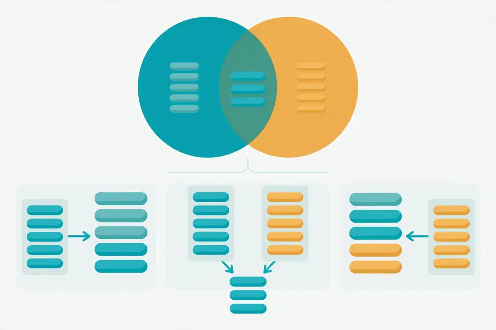
An inner join keeps only rows that match in both tables:

SELECT p.full_name, m.visit_no, m.weight_kg
FROM participants p
INNER JOIN measurements m ON m.part_id = p.part_id
ORDER BY p.full_name, m.visit_no
LIMIT 4;

Expected:

full_name	visit_no	weight_kg
Ayesha Rahman	0	78.5
Ayesha Rahman	1	78.0
Ayesha Rahman	2	77.8
Ayesha Rahman	3	77.5

Anatomy of the join:

• participants p — the table alias p. With joins, aliases are not cosmetic; they are how you say which table's column you mean.
• ON m.part_id = p.part_id — the join condition: match rows where the foreign key equals the primary key. This is the single most important line in join SQL. Get it wrong and everything downstream is fiction.
• INNER is the default; JOIN alone means INNER JOIN. Write INNER explicitly while learning.

The Venn diagram above shows it visually: two circles (the tables), and the inner join is the overlap — rows present in both.

Joining three tables: the study question

Here is the canonical research query — mean weight change by treatment group. It needs all four tables:

SELECT g.group_name,
       COUNT(DISTINCT p.part_id) AS n_participants,
       ROUND(AVG(m.weight_kg), 1) AS mean_weight
FROM treatment_groups g
INNER JOIN assignments a ON a.group_id = g.group_id
INNER JOIN participants p ON p.part_id = a.part_id
INNER JOIN measurements m ON m.part_id = p.part_id
WHERE m.visit_no IN (0, 3)
GROUP BY g.group_name
ORDER BY g.group_name;

Expected:

group_name	n_participants	mean_weight
control	4	78.3
diet	4	80.9
exercise	4	79.3

Hmm — that averages baseline and final together, which is not quite the analysis we want. The change needs baseline and final side by side. That requires joining measurements to itself — a self join, coming up below. First, the join types.

LEFT JOIN: keep everything on the left

A left join keeps all rows from the left table, filling NULLs where the right table has no match:

-- All participants and their visit-3 weight (NULL if they missed it)
SELECT p.full_name, m.weight_kg AS final_weight
FROM participants p
LEFT JOIN measurements m
  ON m.part_id = p.part_id AND m.visit_no = 3
ORDER BY p.full_name;

Expected (excerpt):

full_name	final_weight
Ayesha Rahman	77.5
Bilal Khan	90.0
Chen Wei	61.2
Danish Ali	NULL
…	…

Danish Ali (P004) missed visit 3 — the inner join would have silently dropped him; the left join shows him with NULL. This is the join you want whenever "everyone in the study" is the denominator, e.g., intention-to-treat style summaries or dropout analysis. In fact, finding dropouts is a left join plus a NULL test:

-- Participants with NO visit-3 measurement (lost to follow-up)
SELECT p.part_id, p.full_name
FROM participants p
LEFT JOIN measurements m
  ON m.part_id = p.part_id AND m.visit_no = 3
WHERE m.part_id IS NULL;
-- Expected: P004 (Danish Ali)

That pattern — LEFT JOIN then WHERE right.key IS NULL — is "find rows in A with no match in B." Memorize it; it appears in data-quality audits constantly.

Note the condition placement subtlety: putting AND m.visit_no = 3 inside the ON clause keeps all participants. If you instead put WHERE m.visit_no = 3, the NULL rows (where visit_no is NULL) get filtered out and your left join silently becomes an inner join. Filter on the right table inside ON for left joins — this is a top-five beginner bug.

RIGHT JOIN and FULL OUTER JOIN

• RIGHT JOIN keeps all rows from the right table. A LEFT JOIN B ≡ B RIGHT JOIN A — just reorder the tables and use LEFT. Most analysts never write RIGHT JOIN; knowing it exists is enough to read others' code.
• FULL OUTER JOIN keeps all rows from both tables, NULL-filling both sides. Use it to reconcile two sources: "which participant IDs are in the enrollment file but not the lab file, and vice versa":

SELECT COALESCE(e.part_id, l.part_id) AS part_id,
       CASE WHEN e.part_id IS NULL THEN 'lab only'
            WHEN l.part_id IS NULL THEN 'enrollment only'
            ELSE 'both' END AS source
FROM enrollment e FULL OUTER JOIN lab_results l ON l.part_id = e.part_id;

Dialect note: MySQL does not support FULL OUTER JOIN directly (emulate with LEFT JOIN ... UNION ... RIGHT JOIN); SQLite added support in version 3.39 (2022). PostgreSQL and SQL Server support it fully.

SELF JOIN: a table joining itself

Sometimes the comparison you need is within one table — each row compared to another row of the same table. Give the table two different aliases and it becomes two logical tables:

-- Weight change from baseline (visit 0) to final (visit 3), per participant
SELECT b.part_id,
       b.weight_kg AS baseline_kg,
       f.weight_kg AS final_kg,
       ROUND(f.weight_kg - b.weight_kg, 1) AS change_kg
FROM measurements b
INNER JOIN measurements f
  ON f.part_id = b.part_id
 AND f.visit_no = 3
 AND b.visit_no = 0
ORDER BY change_kg;

Expected (first 4):

part_id	baseline_kg	final_kg	change_kg
P005	85.0	80.0	-5.0
P006	95.0	90.0	-5.0
P010	98.0	93.0	-5.0
P011	74.0	69.5	-4.5

(The full ordering: P005/P006/P010 −5.0, P011/P012 −4.5, P008/P009 −4.0, P007 −3.0, P001/P002 −1.0, P003 −0.8; P004 excluded — no visit 3.)

This is the before/after analysis pattern: join the table to itself on the entity key, with each alias filtered to a different time point. It generalizes to any paired comparison — pre/post surveys, matched cases and controls, month-over-month sensor readings.

The accidental cross join

Forget the ON clause and you get a cross join — every row × every row:

-- NEVER do this accidentally: 12 participants × 44 measurements = 528 rows
SELECT COUNT(*) FROM participants, measurements;

540 rows of meaningless combinations. The comma syntax (FROM a, b) is an implicit cross join and a relic — always use explicit JOIN ... ON. If a query returns far more rows than expected, a missing or wrong ON condition is suspect #1. Always sanity-count after joining: SELECT COUNT(*) before and after, and know what the count should be.

Join diagnostics checklist

When join results look wrong, check in this order:

1. Row count. More rows than expected? The join key is not unique on one side (fan-out). Fewer? Inner join dropped non-matching rows — did you want LEFT?
2. The ON condition. Is it the right key pair? A join on city instead of part_id produces plausible-looking garbage.
3. Duplicates in the key. SELECT part_id, COUNT(*) FROM assignments GROUP BY part_id HAVING COUNT(*) > 1; — if a "one" side has duplicates, every join through it multiplies rows.
4. NULL keys. NULL never matches NULL in a join — rows with NULL keys vanish from inner joins silently.

ON vs USING: the shorthand

When the join columns have the same name in both tables, USING is cleaner than ON:

-- These are equivalent:
SELECT p.full_name, m.weight_kg
FROM participants p JOIN measurements m ON m.part_id = p.part_id;

SELECT full_name, weight_kg
FROM participants JOIN measurements USING (part_id);

Bonus: USING outputs the join column once (no p.part_id vs m.part_id ambiguity), which also fixes the "ambiguous column" error class. NATURAL JOIN goes further — joins on all same-named columns automatically — but it's dangerous (a future column added to both tables silently changes the join). Professionals use ON or USING, never NATURAL JOIN.

Non-equi joins: matching on ranges, not equality

Joins don't require =. A non-equi join matches on inequalities — e.g., assigning each measurement to the enrollment period it falls in, or banding values:

-- Categorize each baseline systolic into a risk band stored in a table
CREATE TABLE risk_bands (band TEXT, lo INTEGER, hi INTEGER);
INSERT INTO risk_bands VALUES ('normal',0,119),('elevated',120,139),('high',140,999);

SELECT m.part_id, m.systolic, b.band
FROM measurements m JOIN risk_bands b
  ON m.systolic BETWEEN b.lo AND b.hi
WHERE m.visit_no = 0
ORDER BY m.systolic;

This pattern — a small "band/lookup table" joined with BETWEEN — replaces nested CASE expressions and keeps the category definitions as data (editable, auditable) rather than buried in code.

Semi-joins and anti-joins: EXISTS as join logic

EXISTS (Chapter 9) is logically a semi-join: "rows in A that have at least one match in B" — without duplicating A rows when B has several matches (an INNER JOIN would multiply them). NOT EXISTS is the anti-join: "rows in A with no match in B." When you need "participants who have any hypertensive reading" (not "hypertensive readings"), the semi-join is the correct, duplication-free tool:

-- Participants with at least one hypertensive reading (one row per participant)
SELECT p.part_id, p.full_name
FROM participants p
WHERE EXISTS (SELECT 1 FROM measurements m
              WHERE m.part_id = p.part_id AND m.systolic >= 140);
-- Expected: P002, P004, P006, P010

An INNER JOIN here would return one row per hypertensive reading — wrong grain for a participant list. Grain discipline (Chapter 8's checklist item 1) is what separates these choices.

How the database actually joins (conceptually)

You don't need to be a database administrator, but knowing the three join strategies explains performance cliffs:

• Nested loop — for each row in A, scan B for matches. Fine when B is tiny or indexed; catastrophic for two huge tables.
• Hash join — build a hash table of B's keys, then probe it with A's rows. The workhorse for large analytical joins.
• Merge join — if both inputs are sorted on the key, zip them together in one pass. Blazing fast, which is why indexes on join keys matter.

The optimizer picks among these automatically. Your job as an analyst is just to give it what it needs: join on indexed key columns (primary/foreign keys usually are), and filter early with WHERE so the join inputs are small. If a join of two big tables is slow, EXPLAIN will show you which strategy was chosen — and then it's a DBA conversation, not an analyst one.

Common errors and fixes

Error	What happened	Fix
ambiguous column name	Both tables have the column; you didn't qualify	p.part_id, m.part_id — always alias-qualify in joins
Row count explodes after join	Join key duplicated on one side, or missing ON	Check key uniqueness; verify ON condition
LEFT JOIN "loses" rows	Filter on right table placed in WHERE instead of ON	Move right-table conditions into the ON clause
invalid reference to FROM-clause entry	Alias used before it's defined	Define aliases in FROM/JOIN, use them after
Join on wrong keys gives plausible garbage	e.g., joined on city — no error, wrong answer	Always join foreign key → primary key; verify with counts

For your research

Every "Table 1: characteristics by group" and every "Figure 2: outcomes over time" in your paper starts as a join. Two habits protect you: (1) comment every join with the relationship — -- one row per participant per visit — so a reader can verify the grain; (2) count at every join step when building a complex query (run the FROM+JOIN alone with COUNT(*) before adding GROUP BY). A paper's numbers are only as trustworthy as its joins, and joins are where silent row-multiplication lives. The self-join before/after pattern in this chapter is directly publishable as a "change from baseline" analysis.

Key takeaways

• INNER keeps matches; LEFT keeps all left rows (NULL-fill right); RIGHT is LEFT reversed; FULL keeps everything from both; SELF joins a table to itself with two aliases.
• The ON condition (foreign key = primary key) is the most important line in the query.
• LEFT JOIN + WHERE right.key IS NULL finds non-matching rows (dropouts, missing records).
• Right-table filters go in ON for outer joins, not WHERE.
• Always count rows before/after joining; fan-out from duplicate keys is the classic silent error.

---

Chapter 9: Subqueries and CTEs — Breaking Hard Problems Down

The problem with one giant query

The Chapter 8 weight-change query answered "change per participant." Now answer the paper's question: "mean weight change by treatment group." You could nest everything into one massive query — and many beginners do, producing an unreadable wall of SQL that nobody (including its author, a month later) can verify. The professional alternative: break the problem into named steps.

Two tools do this: subqueries (a query inside another query) and CTEs — Common Table Expressions, the WITH clause. CTEs are the tool you will actually use; subqueries are the concept underneath.

Subqueries: queries inside queries

A subquery is a SELECT in parentheses used as a building block. Three positions:

1. In WHERE — "rows matching a computed set":

-- Participants whose baseline systolic was above the overall baseline mean
SELECT part_id, systolic
FROM measurements
WHERE visit_no = 0
  AND systolic > (SELECT AVG(systolic) FROM measurements WHERE visit_no = 0);

Expected: P002 (145), P004 (150), P006 (142), P010 (152) — the four above the mean of ≈136.6. The inner query returns one value; the outer compares against it. This is a scalar subquery.

2. In FROM — "aggregate, then aggregate again":

-- Mean OF per-participant mean steps (two-level aggregation)
SELECT ROUND(AVG(mean_steps), 0) AS overall_mean_steps
FROM (
    SELECT part_id, AVG(steps) AS mean_steps
    FROM measurements
    GROUP BY part_id
) AS per_person;

The inner query makes a temporary table (one row per participant with their mean steps); the outer averages those. You cannot do this in one GROUP BY — SQL needs the intermediate step materialized, and the subquery provides it. (Expected ≈ 4903.)

3. In SELECT — "a computed column per row": (use sparingly; often slow)

SELECT full_name,
       (SELECT COUNT(*) FROM measurements m WHERE m.part_id = p.part_id) AS n_visits
FROM participants p;

This is a correlated subquery — it references the outer query (p.part_id) and runs once per row. Correct but slow on big tables; a GROUP BY + join usually beats it.

EXISTS and NOT EXISTS: the safe membership tests

IN with a subquery has the NULL-poisoning problem from Chapter 4. EXISTS / NOT EXISTS do not — they test for the existence of matching rows, and NULLs cannot poison them:

-- Participants with no visit-2 measurement (missed the week-8 follow-up)
SELECT p.part_id, p.full_name
FROM participants p
WHERE NOT EXISTS (
    SELECT 1 FROM measurements m
    WHERE m.part_id = p.part_id AND m.visit_no = 2
);
-- Expected: P002 (Bilal Khan), P007 (Gul Naz) — the two with no visit-2 row

Read it as plain English: "participants where there does NOT EXIST a visit-2 measurement." SELECT 1 inside EXISTS is idiom — the content is irrelevant, only existence matters. Prefer NOT EXISTS over NOT IN whenever the subquery might return NULLs. Prefer EXISTS over IN for large tables — the database can stop searching at the first match.

CTEs: named steps with WITH

A CTE gives a subquery a name and puts it before the main query, so logic reads top-to-bottom:

WITH baseline AS (
    -- Step 1: one row per participant, baseline weight
    SELECT part_id, weight_kg AS w0
    FROM measurements WHERE visit_no = 0
),
final AS (
    -- Step 2: one row per participant, final weight
    SELECT part_id, weight_kg AS w3
    FROM measurements WHERE visit_no = 3
),
change AS (
    -- Step 3: join them into change per participant
    SELECT b.part_id, b.w0, f.w3,
           ROUND(f.w3 - b.w0, 1) AS change_kg
    FROM baseline b INNER JOIN final f ON f.part_id = b.part_id
)
-- Step 4: average the change by treatment group
SELECT g.group_name,
       COUNT(*) AS n,
       ROUND(AVG(c.change_kg), 1) AS mean_change_kg
FROM change c
INNER JOIN assignments a ON a.part_id = c.part_id
INNER JOIN treatment_groups g ON g.group_id = a.group_id
GROUP BY g.group_name
ORDER BY mean_change_kg;

Expected:

group_name	n	mean_change_kg
exercise	4	-4.5
diet	4	-4.3
control	3	-0.9

There is your paper's headline result: the exercise group lost a mean of 4.5 kg, diet 4.3 kg, control 0.9 kg. (Control n=3 because P004 missed the final visit — the inner join in step 3 dropped him; a LEFT-join version would show him with NULL change, and your methods text should say which you used.)

Each CTE is independently testable: run WITH baseline AS (...) SELECT * FROM baseline; to verify step 1 before building step 2. That testability is the entire point — a CTE chain is a lab notebook: dated, ordered, checkable steps instead of one inscrutable query.

You can also chain CTEs with commas (as above) and reference earlier CTEs in later ones. A CTE can even be recursive (a CTE that references itself) — used for hierarchies like organizational charts or citation trees. Syntax:

WITH RECURSIVE subordinates AS (
    SELECT employee_id, manager_id, 1 AS level FROM employees WHERE manager_id IS NULL
    UNION ALL
    SELECT e.employee_id, e.manager_id, s.level + 1
    FROM employees e INNER JOIN subordinates s ON s.employee_id = e.manager_id
)
SELECT * FROM subordinates;

You will rarely need recursion in analysis, but recognizing it lets you read others' code.

CTEs vs subqueries vs temp tables vs views

Tool	Scope	Best for
Subquery in FROM/WHERE	One query	Small one-off building blocks
CTE (WITH)	One query	Multi-step logic you want readable and testable
Temp table	Session	Huge intermediates reused across many queries
View	Database (persistent)	A "virtual table" reused across sessions and users

Rule of thumb: reach for CTEs first. Graduate to temp tables when a CTE is recomputed expensively many times; graduate to views when the logic is a permanent part of the project ("the analysis-ready cohort") that collaborators should reuse.

Scalar subqueries in the SELECT list

A subquery returning exactly one value can sit in the SELECT list as a computed column — e.g., each participant's baseline weight next to their group's mean baseline weight:

SELECT p.part_id,
       m.weight_kg AS baseline_kg,
       (SELECT ROUND(AVG(m2.weight_kg),1)
        FROM measurements m2
        JOIN assignments a2 ON a2.part_id = m2.part_id
        WHERE m2.visit_no = 0 AND a2.group_id = a.group_id) AS group_mean_kg
FROM participants p
JOIN measurements m ON m.part_id = p.part_id
JOIN assignments a ON a.part_id = p.part_id
WHERE m.visit_no = 0
ORDER BY p.part_id
LIMIT 3;

Expected (first 3):

part_id	baseline_kg	group_mean_kg
P001	78.5	79.9
P002	91.0	79.9
P003	62.0	79.9

(Correlated: the inner query references a.group_id from the outer row.) Correct and readable — but it executes once per row, so on 10 million rows prefer the GROUP BY + join rewrite. Use scalar subqueries for small-to-medium results where clarity beats speed.

Derived tables must be aliased

Every subquery in FROM needs an alias — the database requires it (AS per_person in Chapter 9's example wasn't decoration). Without one: subquery in FROM must have an alias (PostgreSQL) or similar. The alias also namespaces the columns: per_person.mean_steps. Same rule applies to CTEs implicitly (the CTE name is the alias).

One CTE, used twice: the recomputation trap

A CTE referenced twice in the main query is typically executed twice (most databases inline CTEs rather than materializing them). For a cheap CTE this is fine; for an expensive one (scanning 100M rows), create a temp table instead:

CREATE TEMP TABLE change AS
    -- ... expensive per-participant change computation ... ;

SELECT ... FROM change ... ;  -- reuse as often as you like
SELECT ... FROM change ... ;

(PostgreSQL 12+ lets you force materialization: WITH change AS MATERIALIZED (...). SQLite and others: use the temp table.) Temp tables vanish when your session ends — perfect scratch space with no cleanup.

The WITH-query shape checklist

Before you call a multi-CTE query done, verify:

1. Each CTE runs standalone and its row count matches expectation.
2. Joins between CTEs are on the right keys (count after each join).
3. The final SELECT's grain is what the paper needs (one row per participant? per visit? per group?).
4. Column names are analysis-ready (aliases a reader understands).
5. The whole thing runs top-to-bottom in a fresh session (no dependency on temp state).

EXISTS vs IN vs JOIN: choosing the membership test

Three ways to ask "participants in group X" — with different performance and correctness profiles:

-- A: IN with subquery (simple; NULL-poison risk on NOT IN)
SELECT full_name FROM participants
WHERE part_id IN (SELECT part_id FROM assignments WHERE group_id = 3);

-- B: EXISTS (NULL-safe; stops at first match — often fastest)
SELECT full_name FROM participants p
WHERE EXISTS (SELECT 1 FROM assignments a
              WHERE a.part_id = p.part_id AND a.group_id = 3);

-- C: INNER JOIN (duplicates outer rows if the subquery has dupes)
SELECT DISTINCT p.full_name FROM participants p
JOIN assignments a ON a.part_id = p.part_id
WHERE a.group_id = 3;

Guidance: use EXISTS for "has at least one" questions (NULL-safe, duplication-free, usually fastest on large tables). Use IN for small static lists (IN ('P001','P002')). Use JOIN when you need columns from both tables. And never use NOT IN with a subquery that might return NULL — that's the Chapter 4 trap, and NOT EXISTS is the escape.

Recursive CTEs: hierarchies and sequences

Chapter 9 introduced WITH RECURSIVE for hierarchies. A second classic use: generating sequences — e.g., the complete list of expected visits (0–3) for the missing-visit audit in Exercise 8:

WITH RECURSIVE visits(n) AS (
    SELECT 0
    UNION ALL
    SELECT n + 1 FROM visits WHERE n < 3
),
expected AS (
    SELECT p.part_id, v.n AS visit_no
    FROM participants p CROSS JOIN visits v
)
SELECT e.part_id, e.visit_no
FROM expected e
LEFT JOIN measurements m
  ON m.part_id = e.part_id AND m.visit_no = e.visit_no
WHERE m.measure_id IS NULL
ORDER BY e.part_id, e.visit_no;
-- Expected: P002/2, P004/1, P004/3, P007/2 — every missing visit

The recursive CTE builds the numbers 0–3; the CROSS JOIN pairs every participant with every expected visit; the LEFT JOIN + NULL test (Chapter 8's pattern) reveals the gaps. This "generate the complete grid, then find holes" technique generalizes to missing dates in time series, missing survey waves, and any completeness audit.

Common errors and fixes

Error	What happened	Fix
WITH query "returns nothing"	Forgot the final SELECT after the CTE definitions	A WITH clause must be followed by a SELECT/INSERT/UPDATE
CTE referenced twice runs twice	CTEs are usually inlined, not materialized	For expensive CTEs used twice, use a temp table instead
NOT IN returns empty unexpectedly	NULL in subquery results	Use NOT EXISTS
Correlated subquery is very slow	Runs once per outer row	Rewrite as GROUP BY + join
Column name collision between CTEs	Two CTEs output same column name; outer SELECT ambiguous	Alias columns distinctly in each CTE

For your research

Reviewers and supervisors can audit a CTE chain step by step — "show me the baseline table," "show me the change table" — which is exactly how methods scrutiny works. Name your CTEs after analysis concepts (baseline, eligible_cohort, change, adjusted), not mechanics (t1, tmp2). A well-named CTE chain often becomes, with light editing, the analysis pipeline description in your Methods section: "Baseline and final weights were extracted (visits 0 and 3), per-participant change computed, and group means compared." Save each major CTE chain as its own .sql file (Chapter 12's documentation practice).

Key takeaways

• Subqueries nest logic; CTEs (WITH) name each step and read top-to-bottom — prefer CTEs for multi-step analysis.
• EXISTS/NOT EXISTS are the NULL-safe membership tests; prefer them over IN/NOT IN with subqueries.
• Correlated subqueries run per-row — correct but potentially slow; GROUP BY + join is the faster idiom.
• Test each CTE independently; name CTEs after analysis concepts.

---

Chapter 10: Window Functions — ROW_NUMBER, RANK, LAG/LEAD, Running Totals

What aggregates cannot do

Aggregates collapse rows: 45 measurements become one mean. But many analysis questions need both — the detail rows and a computation across them. "Rank participants by weight loss." "Compare each visit to the previous one." "Show the running total of enrollments over time." Doing these with GROUP BY is awkward or impossible, because GROUP BY destroys the rows you still need.

Window functions solve this: they compute across a window of related rows while keeping every row. The result has the same number of rows as the input, plus new computed columns.

The syntax that unlocks everything:

FUNCTION(...) OVER (
    PARTITION BY <grouping columns>   -- like GROUP BY, but rows are kept
    ORDER BY <ordering columns>       -- defines the sequence within each group
    ROWS/RANGE <frame>                -- which rows count (for totals)
)

PARTITION BY divides rows into groups (like GROUP BY); ORDER BY sequences them; the function then computes per row looking at its partition.

ROW_NUMBER and RANK: numbering and ranking rows

-- Rank participants by final-visit weight (heaviest = rank 1)
SELECT part_id, weight_kg,
       ROW_NUMBER() OVER (ORDER BY weight_kg DESC) AS rn,
       RANK()       OVER (ORDER BY weight_kg DESC) AS rnk,
       DENSE_RANK() OVER (ORDER BY weight_kg DESC) AS dense_rnk
FROM measurements
WHERE visit_no = 3
ORDER BY weight_kg DESC;

Expected (first 4):

part_id	weight_kg	rn	rnk	dense_rnk
P010	93.0	1	1	1
P002	90.0	2	2	2
P006	90.0	3	2	2
P012	81.5	4	4	3

Three functions, three tie philosophies:

• ROW_NUMBER — 1, 2, 3, 4… never ties. Ties are broken arbitrarily. Use for "top N per group" (with a subquery filter — window functions can't go in WHERE, see below).
• RANK — 1, 2, 2, 4… ties share a rank, then the numbering skips. This is competition ranking ("two people tied for 2nd, next is 4th").
• DENSE_RANK — 1, 2, 2, 3… ties share, no skipping.

The classic use — top-N per group — needs a subquery because window functions execute after WHERE (logical order again):

-- Heaviest measurement per participant (their baseline, usually)
WITH ranked AS (
    SELECT part_id, visit_no, weight_kg,
           ROW_NUMBER() OVER (PARTITION BY part_id ORDER BY weight_kg DESC) AS rn
    FROM measurements
)
SELECT part_id, visit_no, weight_kg
FROM ranked
WHERE rn = 1
ORDER BY part_id;

PARTITION BY part_id restarts numbering for each participant — "rank within each participant." Expected: 12 rows, mostly visit 0 (P006's heaviest is visit 0 at 95.0; everyone's max is their earliest visit since all lost weight — a nice internal validity check of the data).

LAG and LEAD: looking at neighboring rows

LAG(col) = the value in the previous row; LEAD(col) = the next row — within the partition's ordering. This is the before/after engine:

-- Visit-to-visit weight change per participant
SELECT part_id, visit_no, weight_kg,
       LAG(weight_kg) OVER (PARTITION BY part_id ORDER BY visit_no) AS prev_weight,
       ROUND(weight_kg - LAG(weight_kg) OVER (PARTITION BY part_id ORDER BY visit_no), 1)
           AS visit_change
FROM measurements
ORDER BY part_id, visit_no
LIMIT 6;

Expected (first 6):

part_id	visit_no	weight_kg	prev_weight	visit_change
P001	0	78.5	NULL	NULL
P001	1	78.0	78.5	-0.5
P001	2	77.8	78.0	-0.2
P001	3	77.5	77.8	-0.3
P002	0	91.0	NULL	NULL
P002	1	90.5	91.0	-0.5

The first row per participant has no previous row → NULL. LAG(col, 2) looks back two rows; LAG(col, 1, 0.0) supplies a default instead of NULL. LEAD is the mirror — "next visit's value," useful for computing durations between events.

Compare with Chapter 8's self-join approach: the self-join compared two fixed visits; LAG compares consecutive rows whatever they are. For irregular visit schedules (P002 missed visit 2), LAG honestly compares visit 3 against visit 1 — the actual previous observation. Whether that is what your analysis wants is a methods decision; the point is the query makes the choice explicit.

Running totals and moving averages: frames

Add a frame clause to aggregate over a sliding window:

-- Cumulative enrollments over time
SELECT enrolled,
       COUNT(*) OVER (ORDER BY enrolled
                      ROWS BETWEEN UNBOUNDED PRECEDING AND CURRENT ROW) AS cumulative_n
FROM participants
ORDER BY enrolled;

Expected: cumulative_n runs 1, 2, 3 … 12 down the enrollment dates. Frame vocabulary:

• ROWS BETWEEN UNBOUNDED PRECEDING AND CURRENT ROW — running total from the start.
• ROWS BETWEEN 2 PRECEDING AND CURRENT ROW — moving 3-point window (moving average: AVG(x) OVER (... ROWS BETWEEN 2 PRECEDING AND CURRENT ROW)).
• RANGE vs ROWS: RANGE groups peers with equal ORDER BY values; ROWS counts physical rows. For dates with duplicates, they differ — know which you need.

A moving average of daily steps per participant smooths noisy wearable data — a genuinely common preprocessing step before plotting:

SELECT part_id, visit_no, steps,
       ROUND(AVG(steps) OVER (PARTITION BY part_id ORDER BY visit_no
                              ROWS BETWEEN 1 PRECEDING AND 1 FOLLOWING), 0) AS ma3_steps
FROM measurements
WHERE steps IS NOT NULL
ORDER BY part_id, visit_no;

More window functions worth knowing

Function	What it does	Research use
NTILE(4)	Divides ordered rows into 4 quartiles	Quartile analysis of a biomarker
FIRST_VALUE(x) / LAST_VALUE(x)	First/last value in the frame	Baseline value on every row (compare-to-baseline column)
CUME_DIST()	Cumulative distribution (0–1)	Percentile of each observation
PERCENT_RANK()	Relative rank (0–1)	Normalized ranking
SUM(x) OVER (...)	Running total	Cumulative enrollment, cumulative dose

Baseline-on-every-row is a quiet superpower for longitudinal analysis:

-- Every visit alongside the participant's baseline weight
SELECT part_id, visit_no, weight_kg,
       FIRST_VALUE(weight_kg) OVER (PARTITION BY part_id ORDER BY visit_no) AS baseline_kg,
       ROUND(weight_kg - FIRST_VALUE(weight_kg) OVER (PARTITION BY part_id ORDER BY visit_no), 1)
           AS change_from_baseline
FROM measurements
ORDER BY part_id, visit_no;

The golden rules of windows

1. Window functions cannot appear in WHERE, GROUP BY, or HAVING — they execute after those clauses (logical order: … WHERE → GROUP BY → HAVING → window functions → SELECT → ORDER BY). Filter on their results via a subquery/CTE, as in the top-N example.
2. PARTITION BY without ORDER BY is legal (order irrelevant, e.g., percent of total: SUM(x) OVER (PARTITION BY group)).
3. ORDER BY without PARTITION BY treats the whole result as one partition.
4. An empty OVER () computes over all rows — e.g., AVG(weight_kg) OVER () puts the grand mean on every row, handy for "value vs. overall mean" columns.

The default frame gotcha

Here is the subtlest trap in window functions. When your OVER has an ORDER BY but no frame clause, and the function is an aggregate (SUM, AVG, COUNT), the database silently applies a default frame: RANGE BETWEEN UNBOUNDED PRECEDING AND CURRENT ROW — a running total, not the whole partition!

-- Surprise: this is a RUNNING average, not the participant's overall average
SELECT part_id, visit_no, weight_kg,
       AVG(weight_kg) OVER (PARTITION BY part_id ORDER BY visit_no) AS avg_so_far
FROM measurements
WHERE part_id = 'P001'
ORDER BY visit_no;

Expected:

part_id	visit_no	weight_kg	avg_so_far
P001	0	78.5	78.5
P001	1	78.0	78.25
P001	2	77.8	78.1
P001	3	77.5	78.2

If you wanted the participant's overall mean on every row, you must say so explicitly — either drop the ORDER BY (OVER (PARTITION BY part_id)) or specify the full frame (ROWS BETWEEN UNBOUNDED PRECEDING AND UNBOUNDED FOLLOWING). Without ORDER BY and without a frame, the default is the whole partition — which is why AVG(x) OVER (PARTITION BY g) behaves intuitively but AVG(x) OVER (PARTITION BY g ORDER BY t) suddenly becomes cumulative. This single default explains a large fraction of "my window function gives weird numbers" questions.

NTILE: quartiles in one line

NTILE(n) divides the ordered partition into n roughly-equal buckets — instant quartile/tertile analysis:

-- Which baseline-weight quartile is each participant in?
SELECT part_id, weight_kg,
       NTILE(4) OVER (ORDER BY weight_kg) AS weight_quartile
FROM measurements
WHERE visit_no = 0
ORDER BY weight_kg;

Expected: P003 (62.0) quartile 1 … P010 (98.0) quartile 4, three participants per quartile. Comparing outcomes by quartile ("did the heaviest quartile lose the most?") is a standard sensitivity analysis, and NTILE builds the grouping variable in one line. Note: with 12 rows and 4 buckets it's exact; with non-divisible counts the earlier buckets get the extra row.

Windows vs GROUP BY: choosing the tool

Question	Tool	Why
Mean weight per group (one row per group)	GROUP BY	You want collapsed output
Each visit's weight plus the participant's mean (one row per visit)	Window	You want detail rows enriched
Rank participants within groups	Window (RANK)	Ranking needs row context
Running total of enrollments	Window (frame)	Cumulative over ordered rows
"Top 3 per group"	Window (ROW_NUMBER) + outer filter	Per-group selection

The one-line test: if the answer should have the same number of rows as the input, use a window function; if it should have fewer rows, use GROUP BY. They compose beautifully — a window function inside a CTE, then GROUP BY over it outside.

Common errors and fixes

Error	What happened	Fix
window functions are not allowed in WHERE	Logical order: windows compute after WHERE	Wrap in CTE/subquery, filter outside
ROW_NUMBER ties look random	No deterministic tiebreak in ORDER BY	Add a unique column last: ORDER BY weight_kg DESC, part_id
RANK skips numbers unexpectedly	That's RANK's definition (1,2,2,4)	Use DENSE_RANK for 1,2,2,3 or ROW_NUMBER for no ties
LAG gives NULL on first row	No previous row exists	Expected — use the 3-arg default LAG(x,1,0) if you need a value
Running total restarts oddly	PARTITION BY splits it; or frame defaults	Check partition; specify the frame explicitly

For your research

Window functions answer the longitudinal questions that make intervention studies interesting: trajectories (LAG/LEAD), rankings (RANK), cumulative exposure (running SUM), and baseline-anchored change (FIRST_VALUE) — all without collapsing the data, so every figure in your paper can be traced row-by-row back to source measurements. When your Methods say "visit-to-visit change was computed," the LAG query is that sentence in executable form. One caution for publication: window-function results depend on ordering, so always include a deterministic tiebreak (primary key last in ORDER BY) — "arbitrary tie-breaking" is not a sentence you want to defend in peer review.

Key takeaways

• Window functions compute across related rows while keeping every row: FUNCTION(...) OVER (PARTITION BY ... ORDER BY ...).
• ROW_NUMBER (no ties), RANK (ties + skips), DENSE_RANK (ties, no skips).
• LAG/LEAD read neighboring rows — the visit-to-visit change engine.
• Frame clauses (ROWS BETWEEN ...) give running totals and moving averages.
• Windows run after WHERE/GROUP BY/HAVING — filter their results in an outer query.

---

Chapter 11: Modifying Data — INSERT, UPDATE, DELETE (Safely)

A different mindset

Everything so far has been reading data. INSERT, UPDATE, and DELETE change it — and changes are permanent. In analysis work you modify data less often than you query it, but you still need it: loading a new data extract, correcting a data-entry error, coding a derived variable, removing test rows. The rule of this chapter: every modification starts with a SELECT that shows exactly what will change.

INSERT: adding rows

You already used INSERT in Chapter 2. Two more forms matter:

Insert with named columns (always prefer this — immune to column-order changes):

INSERT INTO participants (part_id, full_name, age, gender, city, enrolled)
VALUES ('P013', 'Nadia Hussain', 39, 'F', 'Karachi', '2026-02-12');

Insert from a query — the workhorse of analysis pipelines (e.g., loading a cleaned extract):

-- Archive baseline measurements into a summary table
CREATE TABLE baseline_summary (
    part_id TEXT PRIMARY KEY,
    w0 REAL,
    sys0 INTEGER
);

INSERT INTO baseline_summary (part_id, w0, sys0)
SELECT part_id, weight_kg, systolic
FROM measurements
WHERE visit_no = 0;
-- 12 rows inserted; verify: SELECT COUNT(*) FROM baseline_summary;

UPDATE: changing existing rows

UPDATE rewrites values in rows matching a WHERE clause:

-- Correct a data-entry error: P002's baseline steps were 2800, not 280
UPDATE measurements
SET steps = 2800
WHERE part_id = 'P002' AND visit_no = 0;

The golden safety rule: write the WHERE as a SELECT first.

-- Step 1: SEE the rows (1 row expected)
SELECT part_id, visit_no, steps FROM measurements
WHERE part_id = 'P002' AND visit_no = 0;

-- Step 2: only then, change them
UPDATE measurements SET steps = 2800
WHERE part_id = 'P002' AND visit_no = 0;

An UPDATE without WHERE updates every row in the table. There is no undo button (outside a transaction — see below). Every database professional has a story about the missing WHERE; make sure yours stays a story you heard, not one you tell.

Bulk updates use the same pattern — e.g., coding a derived variable:

-- Add a column, then fill it from existing data
ALTER TABLE measurements ADD COLUMN bmi REAL;

UPDATE measurements
SET bmi = ROUND(weight_kg / POWER(1.70, 2), 1)  -- placeholder height!
WHERE weight_kg IS NOT NULL;

(BMI needs real heights, which our study table lacks — the technique is what matters: ALTER TABLE ... ADD COLUMN, then a set-based UPDATE. One statement updates all 45 rows; no loops, no spreadsheet fill-down.)

DELETE: removing rows

-- Remove test/duplicate rows, after verifying with SELECT
SELECT * FROM measurements WHERE part_id = 'TEST';
DELETE FROM measurements WHERE part_id = 'TEST';

DELETE removes rows; TRUNCATE TABLE measurements removes all rows instantly (faster, usually non-transactional — check your dialect); DROP TABLE measurements removes the table itself. In analysis, prefer DELETE with a precise WHERE; TRUNCATE and DROP are for scratch tables you own completely.

Foreign keys protect you: try DELETE FROM participants WHERE part_id = 'P001' and the database refuses — measurements still reference P001. That refusal is the database doing its job. To truly remove a participant you must delete child rows first (or define the foreign key with ON DELETE CASCADE, which auto-deletes children — powerful and dangerous; use deliberately).

Transactions: the undo button

Wrap risky work in a transaction — a set of statements that succeed or fail together:

BEGIN;  -- or START TRANSACTION;

UPDATE measurements SET weight_kg = weight_kg * 0.453592
WHERE part_id = 'P001';   -- suppose this was a mistake (wrong unit conversion!)

-- Check the damage:
SELECT part_id, weight_kg FROM measurements WHERE part_id = 'P001';

ROLLBACK;  -- undo everything since BEGIN. Crisis averted.
-- (COMMIT; would have made it permanent.)

Workflow for any bulk modification: BEGIN → run statements → SELECT to verify → COMMIT if correct, ROLLBACK if not. Some tools auto-commit every statement (SQLite's default in some interfaces, MySQL's default) — know your tool's behavior before you need it. For a researcher, the practical takeaway: do destructive work on a copy. CREATE TABLE measurements_backup AS SELECT * FROM measurements; takes one line and has saved more analyses than any other single statement.

UPSERT: insert, or update if it exists

Field data arrives in batches, and re-importing a batch shouldn't create duplicates. Upsert = "insert this row, but if the key already exists, update it instead":

-- PostgreSQL / SQLite:
INSERT INTO participants (part_id, full_name, age, gender, city, enrolled)
VALUES ('P001', 'Ayesha Rahman', 35, 'F', 'Karachi', '2026-01-12')
ON CONFLICT (part_id) DO UPDATE SET age = EXCLUDED.age;
-- Updates Ayesha's age to 35 instead of failing on duplicate key

-- MySQL:
-- INSERT INTO participants (...) VALUES (...)
-- ON DUPLICATE KEY UPDATE age = VALUES(age);

ON CONFLICT DO NOTHING is the gentler variant — silently skip duplicates, perfect for idempotent re-imports ("run the load script twice, get the same database"). For research data pipelines that re-run nightly, upsert is the difference between a robust load and a 3 a.m. duplicate-key failure.

RETURNING: see what changed

PostgreSQL and SQLite let an INSERT/UPDATE/DELETE return the affected rows — no second query needed:

UPDATE measurements
SET steps = 2800
WHERE part_id = 'P002' AND visit_no = 0
RETURNING part_id, visit_no, steps;
-- Shows you the changed row immediately: P002 | 0 | 2800

Use it in cleaning scripts as a built-in audit log: every modification statement shows exactly what it touched. (MySQL lacks RETURNING; SQL Server uses an OUTPUT clause.)

DELETE and UPDATE driven by another table

"Delete all measurements for participants who withdrew" — the condition lives in another table. Dialects differ:

-- Portable (subquery):
DELETE FROM measurements
WHERE part_id IN (SELECT part_id FROM withdrawals);

-- PostgreSQL / MySQL (join syntax):
-- DELETE m FROM measurements m JOIN withdrawals w ON w.part_id = m.part_id;

The subquery form works everywhere — prefer it in shared research code. And the safety rule still applies: run the subquery as a SELECT first, eyeball the rows, then delete.

The scratch-table workflow

For experimental transformations, never work on the real table. CREATE TABLE ... AS SELECT (CTAS) snapshots data in one statement:

-- A sandbox copy to experiment on freely
CREATE TABLE measurements_sandbox AS SELECT * FROM measurements;

-- ... try your risky UPDATEs here ...

-- Promote it when correct, or drop it when not
DROP TABLE measurements_sandbox;

CTAS is also how analysts create "analysis-ready" tables: CREATE TABLE analysis_cohort AS <your cohort query> materializes the cohort once, so twenty downstream queries share identical input — and the CTAS statement is the cohort definition, documented and rerunnable.

Bulk updates from another table

"Apply corrected step counts from a staging table to the measurements" — the new values live elsewhere. Dialects differ in spelling, but the subquery form is portable:

-- Portable: correlated subquery in SET
UPDATE measurements m
SET steps = (SELECT s.steps FROM staging_steps s
             WHERE s.part_id = m.part_id AND s.visit_no = m.visit_no)
WHERE EXISTS (SELECT 1 FROM staging_steps s
              WHERE s.part_id = m.part_id AND s.visit_no = m.visit_no);

-- PostgreSQL / SQLite (UPDATE...FROM):
-- UPDATE measurements m SET steps = s.steps
-- FROM staging_steps s WHERE s.part_id = m.part_id AND s.visit_no = m.visit_no;

Bulk updates are where the SELECT-first rule pays for itself many times over: preview the new values per row (SELECT part_id, visit_no, <new expr> AS new_steps ...) before running the UPDATE, and verify counts after (how many rows changed? does it match the preview?).

Soft deletes: why researchers rarely DELETE

In research, deleting participant data is often unethical or non-compliant — ethics approvals typically require retaining source data. The alternative is a soft delete: a flag column marking rows as excluded, keeping them recoverable and auditable:

ALTER TABLE measurements ADD COLUMN excluded BOOLEAN DEFAULT FALSE;
ALTER TABLE measurements ADD COLUMN exclusion_reason TEXT;

-- "Delete" P004's questionable visit-2 reading — reversibly, with a reason
UPDATE measurements
SET excluded = TRUE, exclusion_reason = 'device malfunction per field notes 2026-03-17'
WHERE part_id = 'P004' AND visit_no = 2;

-- All analysis queries then filter:
SELECT AVG(weight_kg) FROM measurements
WHERE visit_no = 0 AND NOT excluded;

The exclusion reason travels with the data — no separate log to lose. Your paper's "excluded measurements" paragraph writes itself from SELECT exclusion_reason, COUNT(*) FROM measurements WHERE excluded GROUP BY exclusion_reason. And un-excluding is one UPDATE, not a restore from backup.

Audit columns: who changed what, when

For shared research databases, add bookkeeping columns to important tables:

ALTER TABLE measurements
    ADD COLUMN created_at TIMESTAMP DEFAULT CURRENT_TIMESTAMP,
    ADD COLUMN created_by TEXT DEFAULT CURRENT_USER,
    ADD COLUMN updated_at TIMESTAMP;

created_at/created_by populate automatically on INSERT. (Keeping updated_at current needs a trigger — ask your DBA, or set it explicitly in UPDATE statements.) When two research assistants enter data and a value looks wrong, audit columns answer "who entered this, and when?" in one query — the difference between a five-minute check and a day of detective work.

Common errors and fixes

Error	What happened	Fix
UPDATE changed all rows	Missing WHERE clause	Restore from backup; always SELECT-first
FOREIGN KEY constraint failed on DELETE	Child rows still reference the row	Delete children first, or reconsider whether deletion is right
INSERT column count mismatch	VALUES list doesn't match column list	Name columns explicitly in INSERT
Changes "disappear" after reconnect	Transaction was rolled back / never committed	COMMIT before closing; check autocommit setting
cannot ALTER TABLE ... ADD COLUMN with NOT NULL	Existing rows would violate it	Add nullable first, UPDATE values, then add constraint

For your research

Data cleaning is analysis, and it must be reproducible. Never clean by hand-editing cells. Instead, write every correction as SQL: the UPDATE that fixed the typo, the DELETE that removed the test rows, the ALTER that added BMI — each in a dated script (cleaning_2026-10-08.sql). Your future self, your supervisor, and your reviewers can then replay the entire cleaning pipeline from raw extract to analysis-ready tables. "We corrected 3 data-entry errors" becomes a verifiable claim, not a memory. And the backup-table habit (_backup suffix, dated) means no cleaning step is ever irreversible.

Key takeaways

• INSERT adds rows (name your columns); UPDATE changes rows; DELETE removes rows.
• SELECT first, then modify — verify the exact affected rows before running UPDATE/DELETE.
• An UPDATE/DELETE without WHERE hits the whole table. There is no undo outside a transaction.
• Use transactions (BEGIN → verify → COMMIT/ROLLBACK) and backup tables before destructive work.
• Foreign keys block deletes that would orphan child rows — that protection is a feature.

---

Chapter 12: SQL for Research — Reproducible Analysis Queries and Query Documentation

From queries to evidence

You now know SQL. This chapter is about using it the way science demands: so that every number in your paper can be regenerated, by someone else, from the raw data, using only your saved queries. That property — reproducibility — is what separates a research query from a casual query.

The uncomfortable truth: most published numbers cannot be regenerated, because the analysis lived in mouse clicks, undocumented spreadsheet formulas, or a Python notebook run out of order. SQL has a structural advantage here — queries are text, text can be saved, saved text can be rerun. This chapter turns that advantage into a practice.

The query file convention

Keep one .sql file per analysis question, named for the question it answers:

study/
├── 00_schema.sql            # CREATE TABLE statements (Chapter 2)
├── 01_load_data.sql         # INSERT statements or COPY commands
├── 02_cleaning.sql          # UPDATE/DELETE corrections, each commented
├── 10_table1_baseline.sql   # Table 1: baseline characteristics by group
├── 11_fig2_trajectories.sql # Figure 2: weight trajectories over visits
├── 12_primary_outcome.sql   # Primary outcome: mean weight change by group
└── README.md                # What each file does, in what order to run

Each file starts with a header comment — the query documentation block:

-- =====================================================================
-- File: 12_primary_outcome.sql
-- Question: What is the mean (SD) weight change from baseline to week 12,
--           by treatment group?
-- Author: A. Rahman, 2026-10-08
-- Database: PostgreSQL 16, database 'wellness'
-- Depends on: 00_schema.sql, 01_load_data.sql, 02_cleaning.sql
-- Paper: Table 2, primary outcome row
-- Notes: P004 excluded (no visit-3 measurement); intention-to-treat
--        sensitivity analysis in 13_sensitivity_itt.sql
-- =====================================================================

WITH baseline AS (
    SELECT part_id, weight_kg AS w0
    FROM measurements WHERE visit_no = 0
),
final AS (
    SELECT part_id, weight_kg AS w3
    FROM measurements WHERE visit_no = 3
),
change AS (
    SELECT b.part_id, (f.w3 - b.w0) AS change_kg
    FROM baseline b JOIN final f USING (part_id)
)
SELECT g.group_name,
       COUNT(*) AS n,
       ROUND(AVG(c.change_kg)::numeric, 1) AS mean_change,
       ROUND(STDDEV(c.change_kg)::numeric, 1) AS sd_change
FROM change c
JOIN assignments a ON a.part_id = c.part_id
JOIN treatment_groups g ON g.group_id = a.group_id
GROUP BY g.group_name
ORDER BY mean_change;

(STDDEV computes the standard deviation — PostgreSQL/MySQL/SQL Server; SQLite needs an extension. The ::numeric cast is PostgreSQL; use CAST(x AS DECIMAL) portably.)

A reviewer reading this file knows: the exact question, the exact code, the exclusions, and where the number appears in the paper. That is documentation that executes.

Commenting inside queries

Comments are the cheapest reproducibility tool. Three places they pay off:

1. Cohort definitions (Chapter 4's rule): -- Eligible: age 30-65, baseline sys >= 130, complete follow-up
2. Magic numbers: WHERE visit_no = 3 -- week-12 final visit (not everyone knows your coding)
3. Deliberate choices: -- LEFT JOIN keeps dropouts visible as NULL (see attrition analysis)

Comment the why, not the what — SELECT age -- selects age helps nobody; HAVING COUNT(*) >= 30 -- minimum n per journal's reporting guideline helps everybody.

Versioning your analysis

When the analysis changes — and it will, after supervisor feedback — do not edit 12_primary_outcome.sql in place and lose the old version. Either:

• Use Git (recommended): git commit after each meaningful change; the history shows exactly what changed and when.
• Or version the filenames: 12_primary_outcome_v1.sql, 12_primary_outcome_v2.sql, with a note on what changed.

Either way, the number in the submitted manuscript must be traceable to exactly one committed query version. "Which query produced Table 2?" should have a one-line answer.

The reproducibility checklist

Before you submit a paper, run this audit on every SQL-derived number:

• [ ] Every table/figure number traces to a saved .sql file (no "I computed it interactively and wrote it down").
• [ ] Each file has the documentation header: question, author, date, dependencies, paper location.
• [ ] Files run in order from raw data to final numbers without errors (test on a fresh database!).
• [ ] Cohort definitions (WHERE clauses) match the Methods text exactly.
• [ ] Rounding is done in the query (ROUND), not by hand during transcription.
• [ ] Exclusions are explicit (who was dropped, why, and where the sensitivity analysis lives).
• [ ] A second person (or future you, in 6 months) can reproduce the numbers from the files alone.

The fresh-database test is the gold standard: create an empty database, run files 00→12 in order, and confirm the output matches the manuscript. If it does, your analysis is genuinely reproducible.

Exporting results for the paper

Queries produce tables; papers need formatted tables. Export cleanly instead of copy-pasting from a terminal:

-- PostgreSQL: CSV export for Excel/Word table building
\copy (SELECT * FROM ...) TO 'table2.csv' WITH CSV HEADER

-- SQLite: 
-- .headers on
-- .mode csv
-- .output table2.csv
-- (run your query)

Name exports after their destination: table2_primary_outcome.csv. Copy-paste from these files into the manuscript — never retype numbers. Retyping is where 4.5 becomes 5.4.

SQL + statistics tools: the handoff

SQL takes you to the analysis-ready dataset; it does not do p-values. The standard research pipeline:

1. SQL — extract, clean, join, aggregate to the analysis dataset (one row per participant with baseline, final, change, group).
2. Export — CSV of exactly that dataset.
3. R / Python / SPSS / Stata — hypothesis tests, regression, plots.
4. SQL again — descriptive tables (Table 1) straight from the database.

Keep the handoff file too (analysis_dataset.csv generation query saved as 09_analysis_dataset.sql). If a statistician asks "how was this variable derived?", the answer is a query, not a memory.

The data dictionary: documenting what columns mean

A query file says how you computed; a data dictionary says what the data means. Keep a DATA_DICTIONARY.md (or a data_dictionary table) alongside your SQL:

Column	Table	Type	Definition	Coding
part_id	participants	TEXT	Unique participant identifier	P001–P012
systolic	measurements	INTEGER	Systolic BP, mmHg, seated after 5 min rest	90–200 valid
visit_no	measurements	INTEGER	Study visit	0=baseline, 1=wk4, 2=wk8, 3=wk12
steps	measurements	INTEGER	Mean daily steps, 7-day recall	NULL = not recorded

Every "what does this column mean?" question a collaborator will ever ask is answered once, here. Reviewers love data dictionaries; they signal a careful study. Generate the skeleton from information_schema.columns (Chapter 2) and fill in the definitions by hand.

README template for the analysis folder

# Karachi Wellness Study — Analysis Queries
Database: PostgreSQL 16, db 'wellness'. Snapshot: data_2026-10-08.csv

Run order:
  00_schema.sql ......... create tables
  01_load_data.sql ...... import CSVs into staging, then main tables
  02_cleaning.sql ....... 3 documented corrections (see header)
  10_table1_baseline.sql  Table 1: baseline characteristics by group
  12_primary_outcome.sql  Table 2: mean weight change by group (primary)

Reproduce: createdb wellness_clean && psql wellness_clean < 00_schema.sql ...
Contact: A. Rahman <a.rahman@university.edu>

A new team member (or you, in two years) reproduces the entire analysis from this file alone. That is the bar.

Citing data and code in your paper

Journals increasingly require data-availability statements. Write yours from the artifacts above:

"The analysis dataset and all SQL queries generating the reported results are archived at [repository link] (query files 00–13, run order in README.md). Table 1 was generated by 10_table1_baseline.sql; the primary outcome (Table 2) by 12_primary_outcome.sql. The database snapshot used for the submitted manuscript is data_2026-10-08.csv (SHA-256: …)."

A hash of the data file (compute with sha256sum) pins the exact snapshot — no ambiguity about "which version of the data."

Archiving for the long term

When the project ends, dump the whole database — schema plus data — into one file:

-- PostgreSQL:  pg_dump wellness > wellness_2026-10-08.sql
-- SQLite:      sqlite3 wellness.db .dump > wellness_2026-10-08.sql
-- MySQL:       mysqldump wellness > wellness_2026-10-08.sql

Store the dump with the query files and the paper manuscript. Ten years from now, anyone can rebuild the entire study database and re-run every number. That is what "reproducible research" actually means — not a vague aspiration, but a folder with a dump, dated queries, and a README.

Common errors and fixes

Error	What happened	Fix
Manuscript number doesn't match re-run	Query was edited after the number was copied	Version queries; re-run everything before submission
"It works on my machine"	Undocumented database state, manual tweaks	Fresh-database test: rebuild from scripts
Collaborator gets different results	Different data snapshot, no version stamp	Stamp exports with date/query version; share the .sql files
Lost which query made Figure 3	Files named query1.sql, final2.sql	Name files for the question; keep the README index

For your research

Start this practice with your current project, not a future one. Today: create the folder, save the schema and the three most important queries with documentation headers, and write the README. It takes an hour and it is the highest-leverage hour in this book — it converts everything you learned from "skills I have" into "evidence I can defend." When your supervisor asks "are you sure about that number?", you will re-run a file instead of re-doing an afternoon.

Key takeaways

• One .sql file per analysis question, named for the question, with a documentation header (question, author, date, dependencies, paper location).
• Comment the why: cohort definitions, magic numbers, deliberate join/filter choices.
• Version queries (Git or v1/v2 filenames); the manuscript number must trace to one version.
• Fresh-database rebuild test is the reproducibility gold standard.
• Export via CSV named for its destination; never retype numbers into the manuscript.

---

Learning Dashboard

This dashboard compresses the book's essential knowledge into reference tables. When you're writing a query and hesitate — "can WHERE see my alias?", "which join keeps the dropouts?", "how do I spell the date function in MySQL?" — come here first. These seven tables answer the questions analysts ask most often, and together they cover roughly 90% of day-to-day analysis SQL. Print them, bookmark them, or copy them into your project's README.

Table D1: Logical order of execution (not the written order!)

Step	Clause	What it does
1	FROM / JOIN	Gather tables and combine them
2	WHERE	Keep rows satisfying row-level conditions
3	GROUP BY	Split surviving rows into groups
4	HAVING	Keep groups satisfying aggregate conditions
5	Window functions	Compute across row windows (ROW_NUMBER, LAG, running SUM)
6	SELECT	Compute output columns, aliases, DISTINCT
7	ORDER BY	Sort the final rows
8	LIMIT / OFFSET	Cap / page the final rows

Why this table matters: it explains every "why can't I do X here?" in SQL — aliases invisible to WHERE (step 6 after step 2), aggregates illegal in WHERE (no groups yet at step 2), window functions illegal in WHERE (step 5 after step 2).

Table D2: JOIN types compared

Join	Keeps	Our study example	When to use it
INNER JOIN	Only matching rows	Participants WITH measurements	Default; both sides must match
LEFT JOIN	All left + matching right (NULLs)	All participants + their visit-3 weight	"Everyone in the cohort" denominators; dropout analysis
RIGHT JOIN	All right + matching left	Rarely written (reorder + LEFT instead)	Reading others' code
FULL OUTER JOIN	All rows from both sides	Reconciling two data sources	"In A not B, in B not A, in both" audits
SELF JOIN	Table joined to itself (two aliases)	Baseline vs final weight per participant	Before/after, pairs, hierarchies
CROSS JOIN	Every combination (usually accidental)	12 × 45 = 540 nonsense rows	Almost never intentional in analysis

Table D3: Function quick-reference

Category	Functions	Chapter
Aggregates	COUNT(*), COUNT(col), COUNT(DISTINCT col), SUM, AVG, MIN, MAX, STDDEV	6
Conditional	CASE WHEN ... THEN ... ELSE ... END, COALESCE(x, default), NULLIF(a, b)	3, 6
Text	UPPER, LOWER, TRIM, LENGTH, SUBSTRING, CONCAT / \|\|	3, 4
Math	ROUND(x, n), POWER, SQRT, ABS, MOD / %	3, 6
Dates (dialect varies!)	PostgreSQL: CURRENT_DATE, AGE(), EXTRACT(YEAR FROM d); SQLite: date('now'), strftime('%Y', d); MySQL: CURDATE(), YEAR(d), DATEDIFF()	3
Ranking windows	ROW_NUMBER(), RANK(), DENSE_RANK(), NTILE(n)	10
Navigation windows	LAG(x), LEAD(x), FIRST_VALUE(x), LAST_VALUE(x)	10
Frame aggregates	SUM(x) OVER (...), AVG(x) OVER (...), COUNT(*) OVER (...)	10

Table D4: WHERE vs HAVING — the definitive distinction

	WHERE	HAVING
Filters	Individual rows	Groups (after aggregation)
Runs	Before GROUP BY	After GROUP BY
Can use aggregates?	No	Yes
Can use SELECT aliases?	No	Sometimes (dialect-dependent)
Example	WHERE visit_no = 0 (baseline rows only)	HAVING COUNT(*) < 12 (incomplete visits)

Table D5: NULL handling cheat sheet

Test	Correct	Wrong
Is missing	WHERE x IS NULL	WHERE x = NULL
Is present	WHERE x IS NOT NULL	WHERE x <> NULL
Not in a set (subquery)	WHERE x NOT IN (SELECT ... WHERE ... IS NOT NULL) or NOT EXISTS	NOT IN with possible NULLs
Default for NULL	COALESCE(x, 0)	Assuming NULL behaves as 0
NULLs in aggregates	Ignored (except COUNT(*))	Assuming they're counted as 0

Table D6: Dialect differences at a glance

Feature	PostgreSQL	MySQL	SQLite	SQL Server
Limit rows	LIMIT 10	LIMIT 10	LIMIT 10	TOP 10 / OFFSET…FETCH
String concat	\|\|	CONCAT()	\|\|	+ / CONCAT()
Case-insensitive LIKE	ILIKE	LIKE (usually)	LIKE (usually)	LIKE (usually)
Current date	CURRENT_DATE	CURDATE()	date('now')	GETDATE() / CAST(GETDATE() AS DATE)
Upsert	ON CONFLICT	ON DUPLICATE KEY	ON CONFLICT	MERGE
Auto-increment PK	GENERATED … IDENTITY	AUTO_INCREMENT	INTEGER PRIMARY KEY	IDENTITY(1,1)
Full outer join	✅	❌ (UNION workaround)	✅ (3.39+)	✅
Window functions	✅	✅ (8.0+)	✅	✅
RETURNING clause	✅	❌	✅	OUTPUT instead
Boolean type	✅ BOOLEAN	TINYINT(1)	INTEGER 0/1	BIT

When writing portable research code, stick to the intersection: standard SELECT/WHERE/GROUP BY/JOIN/CTEs/window functions, and isolate the dialect-specific rows above behind comments.

Table D7: The analyst's query recipes

Question	Pattern	Chapters
How many rows? Any missing?	COUNT(*) vs COUNT(col)	5, 6
Who is in the cohort?	WHERE with parenthesized criteria + COUNT(*) at each step	4
Break it down by group	GROUP BY + aggregates + n per group	7
Change from baseline	Self-join (fixed visits) or LAG (consecutive visits)	8, 10
Top N per group	ROW_NUMBER() in CTE + outer filter	10
Rows in A missing from B	LEFT JOIN + WHERE b.key IS NULL, or NOT EXISTS	8, 9
Running total / moving average	Window frame ROWS BETWEEN …	10
Multi-step analysis	WITH chain of named CTEs, tested step by step	9
Reproducible number for a paper	Documented .sql file + fresh-database rebuild test	12

---

Glossary

• Aggregate function — a function (COUNT, SUM, AVG, MIN, MAX) that collapses many rows into one value; all except COUNT(*) ignore NULLs.
• Alias — a temporary rename for a column (AS) or table, making queries readable and disambiguating joins.
• Cardinality — the numerical relationship between tables (one-to-many, many-to-many); determines whether joins multiply rows.
• CASE expression — SQL's if-then-else; derives categorized columns from raw values.
• CHECK constraint — a rule on a column's allowed values, enforced at insert/update time (e.g., age between 0 and 120).
• Correlated subquery — a subquery referencing the outer query, executed once per outer row; correct but often slow.
• CTE (Common Table Expression) — a named temporary result defined with WITH; breaks multi-step analysis into readable, testable steps.
• Data type — the kind of value a column holds (INTEGER, TEXT, DATE, REAL, BOOLEAN).
• Dialect — a database vendor's variant of SQL (PostgreSQL, MySQL, SQLite, SQL Server); core syntax shared, details differ.
• DISTINCT — keyword removing duplicate rows from results; COUNT(DISTINCT col) counts unique values.
• Foreign key — a column referencing another table's primary key; the glue that makes joins meaningful.
• Frame clause — the ROWS/RANGE BETWEEN specification in a window function defining which rows the window covers (running totals, moving averages).
• GROUP BY — clause splitting rows into groups for per-group aggregation; every bare SELECT column must appear in it.
• HAVING — clause filtering groups after aggregation (WHERE filters rows before it).
• Index — a database structure speeding up lookups on a column; analysts benefit automatically, administrators create them.
• JOIN — operation combining rows from two tables on a matching condition (ON clause), typically foreign key = primary key.
• NULL — the marker for missing/unknown value; not zero, not empty string; never equal to anything including itself.
• Normalization — organizing data into related tables to eliminate redundancy; the reason analysis needs joins.
• PARTITION BY — window-function clause dividing rows into groups for independent computation, without collapsing rows.
• Primary key — the column(s) uniquely identifying each row; never NULL, never duplicated.
• Query — a SQL statement (usually SELECT) asking the database a question; every query returns a table.
• Referential integrity — the guarantee (via foreign keys) that references between tables always point to real rows.
• Reproducibility — the property that saved queries regenerate a paper's numbers exactly from raw data.
• Schema — the structure of a database: tables, columns, types, keys, and constraints.
• Subquery — a SELECT nested inside another statement (in WHERE, FROM, or SELECT).
• Transaction — a group of statements executed atomically (all-or-nothing), with COMMIT making changes permanent and ROLLBACK undoing them.
• Window function — a function (ROW_NUMBER, RANK, LAG, SUM() OVER...) computing across a set of related rows while keeping every row.
• Logical order of execution — the actual evaluation sequence (FROM → WHERE → GROUP BY → HAVING → windows → SELECT → ORDER BY → LIMIT), distinct from written order.
• Sargable — a WHERE condition the database can evaluate with an index (e.g., enrolled >= '2026-02-01'); wrapping a column in a function (strftime('%m', enrolled) = '02') is usually non-sargable and slow on large tables.
• Upsert — an INSERT that updates the row instead of failing when the key already exists (ON CONFLICT / ON DUPLICATE KEY); makes data-loading scripts idempotent.
• CTAS (CREATE TABLE AS SELECT) — creating a table from a query's results in one statement; used for sandbox copies and materializing analysis-ready tables.
• De-identification — replacing direct identifiers with study codes (and storing the mapping separately under restricted access) so analysis datasets can't identify participants.
• Collation — the rules a database uses to compare and sort text (case sensitivity, accent handling); explains why sorted text sometimes looks "wrong."
• Lakehouse — a modern architecture letting you query raw files in a data lake with SQL; the analyst's interface stays SQL even at massive scale.

---

Practice Exercises

Work against the Karachi Wellness Study schema from Chapter 2 (all data as inserted there). Write and run each query; check your results against the expected answers given.

Exercise 1 (easy). List the full name, age, and city of all participants from Karachi, sorted alphabetically by name. (Expected: 6 rows — Ayesha Rahman, Bilal Khan, Danish Ali, Gul Naz, Iqra Sheikh, Kiran Malik.)

Exercise 2 (easy). Find all baseline (visit 0) measurements with systolic ≥ 140. Show part_id and systolic, sorted by systolic descending. (Expected: 4 rows — P010 152, P004 150, P002 145, P006 142.)

Exercise 3 (moderate). For each city, show the number of participants and their mean age (1 decimal). Exclude cities with fewer than 2 participants. (Expected: Karachi 6, 36.7; Lahore 3, 43.0; Islamabad 3, 42.7.)

Exercise 4 (moderate). Categorize every baseline measurement with a CASE expression: 'hypertensive' (systolic ≥ 140 OR diastolic ≥ 90), 'elevated' (systolic ≥ 120), else 'normal'. Count participants per category. (Expected: hypertensive 5, elevated 6, normal 1. Hint: evaluate hypertensive first.)

Exercise 5 (moderate). Show each participant's name, group name, and number of recorded visits, including participants' full visit counts even where visits were missed. Sort by n_visits ascending, then name. (Expected: 12 rows; P004 has 2 visits, P002 and P007 have 3, everyone else has 4. Requires a LEFT JOIN from participants to measurements plus GROUP BY.)

Exercise 6 (challenging). Compute the mean visit-to-visit weight change per treatment group using LAG. Steps: (a) in a CTE, compute per-row visit_change with LAG partitioned by participant; (b) join to assignments/groups; (c) average the non-NULL changes per group. (Expected approximately: control −0.42, diet −1.55, exercise −1.50 kg per visit. Small differences from rounding choices are fine — document yours.)

Exercise 7 (challenging). Find participants whose final-visit (visit 3) weight is in the top 3 within their own treatment group. Use RANK() partitioned by group and filter ranks ≤ 3. (Expected: 9 rows — 3 per group. In control: P002 90.0, P004 has no visit 3... think carefully about who qualifies! Control visit-3 rows: P001 77.5, P002 90.0, P003 61.2 — only 3 exist, so all qualify.)

Exercise 8 (challenging). Identify "incomplete follow-up" participants (fewer than 4 measurements) and, for each, list which visit numbers are missing. (Hint: generate the expected visits 0–3 per participant — e.g., CROSS JOIN participants with a 4-row values table — then LEFT JOIN measurements and keep the NULLs. Expected missing: P002 visit 2; P004 visits 1, 3; P007 visit 2.)

Exercise 9 (research-oriented). Build the analysis dataset for the paper's primary outcome: one row per participant with columns part_id, group_name, age, gender, baseline weight, final weight, and weight change. Save it as a documented .sql file (header block per Chapter 12) that exports to CSV. Then write the two sentences for your Methods section describing exactly how the dataset was derived, including the exclusion rule you applied.

Exercise 10 (research-oriented). Write a "Table 1" query: baseline characteristics (n, mean age, % female, mean systolic, mean weight) by treatment group, with a documented .sql file and README entry. Then deliberately introduce one data error (on a copy of the database), re-run your query files from scratch on the copy, and confirm the table regenerates with the changed value — demonstrating your pipeline is truly reproducible. Write a three-line "reproducibility statement" suitable for a journal's data-availability section.

---

References

[1] A. Beaulieu, Learning SQL, 3rd ed. Sebastopol, CA, USA: O'Reilly Media, 2020.

[2] J. Celko, Joe Celko's SQL for Smarties: Advanced SQL Programming, 5th ed. Cambridge, MA, USA: Morgan Kaufmann, 2014.

[3] PostgreSQL Global Development Group, "PostgreSQL 16 documentation," 2023. [Online]. Available: https://www.postgresql.org/docs/16/

[4] Oracle Corporation, "MySQL 8.0 reference manual," 2023. [Online]. Available: https://dev.mysql.com/doc/refman/8.0/en/

[5] SQLite Consortium, "SQLite documentation: SQL syntax," 2024. [Online]. Available: https://www.sqlite.org/lang.html

[6] C. J. Date, SQL and Relational Theory: How to Write Accurate SQL Code, 3rd ed. Sebastopol, CA, USA: O'Reilly Media, 2015.

[7] R. Ramakrishnan and J. Gehrke, Database Management Systems, 3rd ed. New York, NY, USA: McGraw-Hill, 2002.

[8] A. Silberschatz, H. F. Korth, and S. Sudarshan, Database System Concepts, 7th ed. New York, NY, USA: McGraw-Hill, 2019.

[9] Microsoft Corporation, "Transact-SQL (T-SQL) reference," 2024. [Online]. Available: https://learn.microsoft.com/en-us/sql/t-sql/

[10] W3Schools, "SQL tutorial," 2024. [Online]. Available: https://www.w3schools.com/sql/ (Useful for quick syntax checks; verify dialect details against vendor docs [3]–[5].)

---

End of Book 22. Next: Book 23 — Python for Data Analysis (pandas).

Where to Go from Here

You now hold the complete extraction-and-summarization layer of research data work. The honest next steps, in order:

1. Use it on real data this week. Take a dataset from your own field — survey responses, lab readings, anything tabular — load it into SQLite or PostgreSQL, and run the Chapter 5 audit on it. Real data teaches what examples can't.
2. Build your query library. Save every useful query with a documentation header (Chapter 12). Within months you'll have a personal toolkit that makes each new project faster.
3. Learn the handoff. Book 23 (pandas) picks up where SQL leaves off: statistical testing, modeling, and visualization of the datasets your queries produce.
4. Go deeper where it matters. If you work with a specific database daily, read its official documentation cover-to-cover on the topics in Dashboard Table D3 — vendor docs [3], [4], [5], [9] are the ultimate reference.

The deepest lesson of this book isn't syntax — it's that a question asked precisely, in text, against well-structured data, gives an answer you can defend. That habit, applied to every table and figure you ever publish, is what makes a researcher trustworthy.