Automating Reports with Python

Book 41 of 50 — AstolixGen Learning Series (Detailed Edition) For researcher and publication students

About This Book

Every business, laboratory, and university department runs on reports: weekly sales summaries, monthly lab statistics, student enrollment figures, grant expenditure statements. Someone, somewhere, opens a spreadsheet, copies numbers, builds charts, writes a summary, and emails a file — and then does it all again next week. This book teaches you how to hand that repetitive work to Python. You will learn to read data from files, databases, and web services; clean and transform it with pandas; draw publication-quality charts with Matplotlib and Seaborn; assemble polished PDF and Excel reports automatically; email them to the right people; and schedule the whole pipeline so it runs while you sleep. No invented theory here — every chapter uses realistic scenarios from small businesses, research labs, and university offices, with short, working code snippets you can adapt. By the end, you will have the skills to design a reporting pipeline that is accurate, reproducible, and maintainable — the same qualities your research is judged by.

Learning objectives: By the end of this book, you will be able to:

• Explain why automated reporting is more accurate, reproducible, and cost-effective than manual reporting, and make the business and research case for it.
• Set up a reliable Python environment with a package manager, virtual environments, and the core reporting libraries.
• Read data from CSV files, Excel workbooks, relational databases, and web APIs into Python.
• Clean, reshape, and aggregate data with pandas, handling missing values, duplicates, and inconsistent formats.
• Create clear, honest charts with Matplotlib and Seaborn, choosing the right chart type for the message.
• Generate professional PDF reports programmatically and automate Excel workbooks with openpyxl.
• Send reports by email automatically with attachments, using safe credential practices.
• Schedule recurring reports with Task Scheduler, cron, and cloud options.
• Decide when a static report is right and when a dashboard is better.
• Build resilient pipelines with error handling, logging, retries, and data validation.
• Take a reporting script from your laptop into production with version control, documentation, and a maintenance plan.

Learning Dashboard

Chapter map

Chapter	Guiding question	Key takeaway
1. Why Automate Reports? The Business and Research Case	What is the real cost of manual reporting, and what does automation change?	Automation converts a fragile weekly chore into a reliable, auditable pipeline — and pays for itself in accuracy and freed time.
2. Setting Up Your Python Reporting Environment	What tools do I need, and how do I install them so they don't break?	A clean install plus virtual environments gives you a reproducible workspace that works on any machine.
3. Reading Data: CSV, Excel, Databases, and APIs	How do I get data from wherever it lives into Python?	pandas and a few connectors let you read almost any structured data source with a few lines of code.
4. Cleaning and Transforming Data with pandas	How do I turn messy raw data into trustworthy numbers?	Systematic cleaning — missing values, duplicates, types, reshaping — is where report quality is really made.
5. Creating Charts with Matplotlib and Seaborn	How do I make charts that are clear, accurate, and honest?	Choose the chart by the message, label everything, and never let decoration distort the data.
6. Building PDF Reports with Python	How do I produce a polished, fixed-layout report file?	Libraries like ReportLab and fpdf2 turn your numbers and charts into professional PDFs without a word processor.
7. Excel Automation with openpyxl	How do I fill and format Excel workbooks automatically?	openpyxl lets Python write, style, and formula-enable spreadsheets that humans can still edit and trust.
8. Sending Reports by Email Automatically	How do reports reach the right inbox on time, every time?	Python's email tools plus app-passwords or service accounts can deliver reports safely — with logging so you know they arrived.
9. Scheduling: Task Scheduler, Cron, and Cloud Options	How do I make it run on its own schedule?	The operating system's scheduler (cron or Task Scheduler) is enough for most cases; cloud schedulers cover the rest.
10. Dashboards vs Static Reports: Choosing Wisely	Should this be a PDF in an inbox or a live dashboard?	Static reports record a moment and travel anywhere; dashboards answer ad-hoc questions. Pick by the decision the reader must make.
11. Error Handling, Logging, and Reliable Pipelines	What happens when the data is wrong, late, or missing?	Fail loudly, log everything, validate inputs, and design so one bad week never corrupts the archive.
12. From Script to Production: Deployment and Maintenance	How do I hand this over so it keeps working after I leave?	Version control, configuration files, documentation, and a maintenance owner turn a script into a system.

Core tools checklist

Tool	What it does	When to use it
Python 3 + pip	The language and its package installer	The foundation for everything in this book
Virtual environments (venv)	Isolated package sets per project	Every project, always — never install reporting packages globally
pandas	Dataframes: reading, cleaning, reshaping, aggregating tabular data	Every reporting pipeline that touches tables
NumPy	Fast numerical arrays under the hood	When you need vectorized math or pandas is too slow
Matplotlib	Fine-grained, publication-style charts	Any chart you must fully control; base layer under Seaborn
Seaborn	Statistical charts with sensible defaults	Quick, attractive exploratory and summary charts
openpyxl	Reading and writing .xlsx files with formatting	When the deliverable is an Excel workbook
ReportLab / fpdf2	Programmatic PDF generation	When the deliverable is a fixed, print-ready PDF
SQLAlchemy / sqlite3	Database connections and queries	When data lives in a relational database
requests	HTTP calls to web APIs	When data comes from a web service or REST API
smtplib + email	Sending email with attachments	Automated delivery of finished reports
cron / Task Scheduler	Operating-system job scheduling	Running the pipeline on a timetable
logging	Standard library logging to files and consoles	Every pipeline, so failures leave a trail

Research fit: how this book serves a researcher's workflow

Book section	Research workflow benefit
Chapters 1–2 (case + setup)	Frames automation as a research skill: reproducibility, audit trails, and time returned to analysis
Chapters 3–4 (reading + cleaning data)	Mirrors the data-wrangling stage of any empirical study; the same pandas skills clean experimental and survey data
Chapter 5 (charts)	Directly improves thesis and journal figures: honest axes, readable labels, export-ready vector graphics
Chapters 6–7 (PDF + Excel)	Produces progress reports for supervisors, funding agencies, and collaborators without manual retyping
Chapters 8–9 (email + scheduling)	Automates weekly lab updates, data-quality digests, and recurring monitoring summaries
Chapter 10 (dashboards vs reports)	Helps you choose the right communication artifact for committees, conferences, and stakeholders
Chapters 11–12 (reliability + deployment)	Teaches the engineering discipline reviewers expect: documented, versioned, reproducible pipelines

Chapter 1: Why Automate Reports? The Business and Research Case

Picture a small textile trading company in Faisalabad. Every Monday morning, the office manager, Sana, opens three Excel files: sales from the point-of-sale system, stock levels from the warehouse spreadsheet, and expenses typed up by the accountant. She copies figures into a summary sheet, builds two charts, writes a short paragraph about the week's performance, saves it as a PDF, and emails it to the owner. The whole ritual takes her about four hours. In a month with five Mondays, that is twenty hours — half a working week — spent on what is essentially copying and pasting. Worse, twice last quarter a typo in a copied cell made the weekly profit look ten times larger than it was, and the owner made purchasing decisions on the wrong number before anyone noticed. Sana is careful and conscientious; the problem is not Sana. The problem is the process. Manual reporting is slow, it is error-prone, and it steals skilled people's time from work that actually needs a human brain.

Now picture a university research lab running a field trial on wheat varieties across twelve farms. Every Friday, a research assistant downloads sensor data, merges it with the week's field observations recorded on paper forms, computes average soil moisture and temperature per plot, draws a few charts, and emails a one-page summary to the principal investigator. It takes three hours, and because the assistant is also writing a thesis, the report sometimes goes out on Monday instead of Friday, and the chart scales change from week to week, making it hard to compare trends. When a journal reviewer later asks, "How exactly were these weekly summaries computed?" nobody can reconstruct the steps precisely, because the steps lived in someone's head and in a spreadsheet with overwritten cells.

These two stories — the trading company and the research lab — are the same story. A recurring information need, a human doing mechanical work to satisfy it, errors creeping in, time draining away, and no reliable record of how the numbers were produced. Automating reports with Python attacks all of these problems at once.

Let us define what we mean. A report is a structured summary of data, prepared for a decision-maker or a record. A manual report is produced by a person operating software step by step. An automated report is produced by a program that reads data, transforms it, visualizes it, formats it, and delivers it, with the human involved only in designing the pipeline and checking the output. The key insight is that the program does the same thing every time. It does not get tired on a Friday afternoon. It does not misread a cell. It does not skip a step because it is in a hurry. And, crucially, the program itself is a record of the method: the code is the recipe, version-controlled and reviewable, so "how were these numbers computed?" always has an answer.

The business case rests on three pillars: time, accuracy, and timeliness. Time is the easiest to measure. If a weekly report takes four hours and your automation reduces the human effort to fifteen minutes of review, you save roughly 195 hours a year on one report — and most organizations have several. Accuracy is harder to measure but more valuable. Studies of spreadsheet practice have long documented that manual spreadsheets contain errors at alarming rates; even careful operators introduce mistakes when copying and reformatting data repeatedly. A coded pipeline eliminates the entire class of transcription errors: the numbers flow from source to output without a human retyping them. What errors remain — wrong source data, a misunderstood business rule — are at least systematic and fixable in one place rather than scattered across dozens of hand-edited files. Timeliness is the third pillar. A scheduled script runs at 6 a.m. whether or not anyone is at their desk, so the Monday report is in the owner's inbox before the Monday meeting, every Monday, even during holidays. Decisions get made on fresh data instead of last week's guesses.

For researchers, there is a fourth pillar that matters even more: reproducibility. Science runs on the principle that another person, given the same data and methods, should reach the same result. A reporting pipeline written in Python is reproducible by construction. The cleaning steps, the aggregation logic, the chart code — all of it is explicit, and all of it can be shared, reviewed, and rerun years later. When a reviewer or a funding agency asks how a figure was produced, you point to the code. When your successor inherits the project, they inherit a working pipeline, not a folder of ambiguously named spreadsheets. Many universities and journals now expect exactly this level of transparency, and the skills in this book transfer directly: the same pandas code that cleans weekly sales cleans survey responses; the same Matplotlib code that draws a revenue chart draws a publication figure.

A realistic example makes the economics concrete. Consider a small private clinic that must send a monthly report to its management: patient visits by department, revenue by service type, outstanding payments, and a comparison with the previous month. The administrator spends six hours a month building it in Excel — 72 hours a year. At a modest loaded cost, that is real money, but the bigger cost is opportunity: those are six hours not spent on patient scheduling, staff coordination, or following up on unpaid bills. A Python pipeline that reads the clinic's billing export, computes the tables, draws the charts, and produces a PDF might take a competent beginner twenty to thirty hours to build and test — a one-time cost. From then on, the monthly effort drops to a few minutes of review. The payback period is measured in months, and the pipeline keeps paying every month after. This is the fundamental arithmetic of automation: a fixed upfront investment replaces a recurring cost, and the recurring cost never comes back.

It is worth being honest about what automation does not do. It does not fix bad data — if the point-of-sale system records the wrong prices, the automated report will faithfully report the wrong prices, just faster. Data quality work remains human work, though automation can help by adding validation checks that flag suspicious values (Chapter 11 covers this). Automation does not replace judgment: the pipeline can compute that revenue fell 12 percent, but deciding why and what to do about it is still the manager's job — which is precisely why we automate, to give managers their time back for thinking. And automation has its own failure modes: a changed file format, a password that expires, a server that goes down. Chapters 9, 11, and 12 are about managing those risks so the pipeline is genuinely reliable rather than a fragile contraption that breaks the first time reality shifts.

There is also a human and organizational dimension. People sometimes fear that automating a report means automating away a job. In practice, in small businesses, labs, and university offices, the person freed from the reporting chore is rarely dismissed; they are redeployed to work the chore was crowding out. Sana the office manager, freed from four hours of copying, can chase late payments or analyze which products are actually profitable — work that grows the business. The research assistant, freed from Friday chart-building, can spend that time on the thesis. Frame automation as removing drudgery, not removing people, and involve the current report-maker in designing the pipeline: they know the edge cases, the quirks of the data, and the readers' real needs better than anyone.

How do you recognize a report worth automating? Look for three signals. First, recurrence: the report is produced on a schedule — daily, weekly, monthly, per semester. Second, structure: the report has a stable format — the same tables, the same charts, the same sections each time, with fresh data. Third, pain: it takes meaningful time, it has produced embarrassing errors, or it is frequently late. A report with all three signals is an ideal candidate. A one-off, free-form analysis is not — automate the repeatable, and keep humans on the novel.

Before writing any code, a good automation project starts with a small piece of homework: document the current manual process. Sit with the person who makes the report and write down each step: where does each input come from, what transformations are applied, what the output looks like, who receives it, and what decisions it informs. This document becomes your specification, your test plan (the pipeline's output must match the manual output on historical data), and later, your handover notes. It also forces a useful conversation: quite often, parts of the manual report exist "because we've always done it that way," and the automation project is a good moment to ask whether anyone actually reads page four.

The rest of this book builds the pipeline step by step, in the order you would actually build it: environment, data reading, cleaning, visualization, report generation in PDF and Excel, email delivery, scheduling, the dashboard question, reliability engineering, and finally production deployment. Each chapter is practical and self-contained, but they connect into one running example you can follow: by Chapter 12 you will have designed a complete automated reporting system, and you will know how to keep it running.

The anatomy of a reporting pipeline

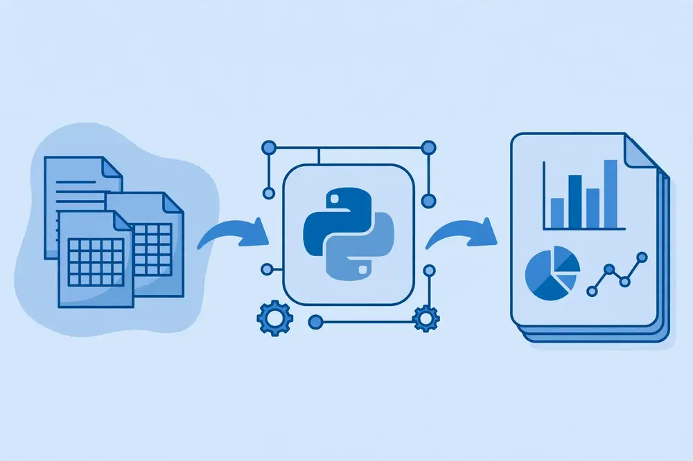
It helps to see the whole machine before building its parts. Every automated reporting pipeline, from a corner shop's weekly summary to a bank's regulatory filing, has the same five stages. Extract: pull raw data from its sources (Chapter 3). Transform: clean, validate, and aggregate it into report-ready numbers (Chapter 4). Visualize: turn key numbers into charts (Chapter 5). Assemble: combine narrative, tables, and charts into the finished document (Chapters 6–7). Deliver: send it to readers on schedule and confirm arrival (Chapters 8–9). Around all five stages run two cross-cutting concerns: reliability (Chapter 11) and lifecycle management (Chapter 12). When something goes wrong — and it will — this anatomy tells you exactly which stage to inspect. A wrong number in the PDF? Check Transform. A missing chart? Check Visualize. An email that never arrived? Check Deliver. Thinking in stages turns debugging from panic into procedure.

Doing the ROI arithmetic honestly

Automation proposals live or die on honest numbers, so let us work one through completely. Take the clinic example from earlier: the administrator spends 6 hours a month on the report, 72 hours a year. Building the pipeline takes, say, 30 hours of focused work (learning included), plus 1 hour a month of maintenance and review — 12 hours a year. Year one: 30 + 12 = 42 hours invested versus 72 hours saved, a net gain of 30 hours. Year two onward: 12 hours invested versus 72 saved, a net gain of 60 hours every year, forever. The payback point arrives around month seven. Two subtleties make the real return even better. First, the manual 72 hours were not just costly but lumpy — they fell in the busiest week of the month, when the administrator was already overloaded; automation smooths that peak. Second, the pipeline's outputs are consistent and auditable in a way the manual report never was, which has value during inspections and funding reviews that never appears in an hours spreadsheet. When you pitch automation to a manager, show both the arithmetic and these second-order benefits — decision-makers respond to the numbers, but they remember the story.

Choosing what to automate first

Rarely can you automate everything at once, so prioritize. Score each candidate report on three axes from 1 to 5: frequency (daily = 5, monthly = 3, quarterly = 1), pain (hours consumed, error history, deadline stress), and stability (how fixed the format and sources are — stable = 5). Multiply the three scores. A weekly report (5) that eats half a day and once caused a bad purchase order (5) with a fixed template and steady data sources (4) scores 100: automate it first. A quarterly narrative report (1) that takes two painful days (4) but changes structure every quarter (2) scores 8: leave it manual for now. This simple scoring does two useful things: it directs your limited building time at the highest return, and it gives stakeholders a transparent rationale when they ask why their report is third in the queue. Start with one high-scoring report, make it a visible success, and the political capital for the next one builds itself.

For your research: Treat your thesis or dissertation data workflow as a reporting pipeline, even if nobody calls it that. Every table in your results chapter and every figure in your paper is a "report" generated from raw data through cleaning and analysis steps. If those steps live in a Python script rather than in manual spreadsheet edits, your work is reproducible, your committee can audit your methods, and revising a chapter after new data arrives becomes a matter of rerunning code instead of redoing weeks of manual work. The business case for automation — time, accuracy, timeliness — applies to your degree timeline too.

Key takeaways:

• Manual reporting is expensive in time, fragile in accuracy, and often late; the cost recurs every cycle while an automation investment is one-time.
• An automated pipeline does the same steps identically every run, eliminating transcription errors and producing an auditable record of the method.
• For researchers, automation's deepest value is reproducibility: code documents exactly how results were produced.
• Automation does not fix bad source data or replace human judgment; it frees humans to do the judgment work.
• Good candidates for automation are recurring, structurally stable, and painful; start by documenting the current manual process as your specification.

Chapter 2: Setting Up Your Python Reporting Environment

Every reliable pipeline starts with a boring foundation: a Python installation you understand, a way to isolate each project's packages, and the right libraries installed deliberately rather than accidentally. This chapter walks through that setup on Windows, macOS, and Linux, because reporting pipelines live in all three worlds — your laptop might run Windows, the lab server might run Linux, and your collaborator might use a Mac. The goal is an environment you can recreate exactly, on any machine, months from now.

Start with Python itself. You need Python 3 — specifically a recent stable version such as 3.11 or 3.12. If Python is already on your machine, check what you have before installing anything new. Open a terminal (Command Prompt or PowerShell on Windows, Terminal on macOS/Linux) and run:

python --version

If that prints something like Python 3.12.3, you are in good shape. If it says Python 2, or the command is not found, download the installer from the official Python website (python.org) for your operating system. On Windows, one checkbox in the installer matters enormously: "Add python.exe to PATH." Check it. Without it, the python and pip commands will not work from the terminal, and you will spend an unhappy afternoon wondering why. On macOS, the system ships an old Python you should leave alone; install a fresh one from python.org or via the Homebrew package manager. On Linux, Python 3 usually comes preinstalled; if not, your distribution's package manager provides it (for example, sudo apt install python3 python3-pip python3-venv on Ubuntu/Debian).

The package installer pip is how you add libraries. Verify it:

pip --version

or, if that fails, python -m pip --version. The python -m pip form is the most reliable because it guarantees you are installing packages for the Python you think you are. Keep pip itself current with python -m pip install --upgrade pip, but do this deliberately rather than blindly — in shared or production environments, upgrade only when you have a reason.

Now the single most important habit in this book: virtual environments. A virtual environment is an isolated Python workspace with its own set of installed packages. Why does this matter? Suppose your sales-report project needs pandas version 2.0, while your thesis analysis needs pandas 1.5 because some old code breaks on the newer version. Installed globally, these two requirements conflict; in separate virtual environments, each project gets exactly what it needs, and neither can break the other. Virtual environments also make your project portable: you can record the exact package list in a file, and anyone — including future-you on a new laptop — can recreate the identical environment.

Creating one is simple. In your project folder:

python -m venv report-env

This creates a report-env directory containing a fresh, isolated Python. To use it, you activate it. On Windows (PowerShell): .\report-env\Scripts\Activate.ps1. On Windows (Command Prompt): report-env\Scripts\activate.bat. On macOS/Linux: source report-env/bin/activate. Your terminal prompt will change to show the environment name, e.g. (report-env). Everything you pip install from now on goes into this environment only. When you are done, deactivate returns you to normal. One rule to internalize: never install project packages outside a virtual environment. The five seconds activation costs will save you from dependency conflicts that cost hours.

With the environment active, install the reporting stack. For this book, the core set is:

pip install pandas openpyxl matplotlib seaborn reportlab fpdf2 requests sqlalchemy

Let us unpack what each of these is for, since you will meet them all in later chapters. pandas is the workhorse for reading and manipulating tabular data. openpyxl reads and writes modern Excel files and is also what pandas uses under the hood for .xlsx files. matplotlib is the foundational charting library; seaborn builds on it with attractive statistical plots. reportlab and fpdf2 are two different PDF generation libraries — you will typically pick one per project (Chapter 6 compares them). requests fetches data from web APIs, and sqlalchemy connects to databases cleanly. You do not need to memorize this list; the Core tools checklist in the Learning Dashboard is your reference.

Pin your versions. After installing, run:

pip freeze > requirements.txt

This writes every package and its exact version into requirements.txt. Commit that file with your project (Chapter 12 covers version control). Six months from now, on a new machine, pip install -r requirements.txt inside a fresh virtual environment reproduces your setup exactly. This single file is the difference between "it worked on my laptop" and a genuinely reproducible pipeline — and reproducibility is a word your thesis committee likes to hear.

Next, choose how you will write code. For learning and development, you have two good options. A code editor such as VS Code (free, with an excellent Python extension) is ideal for writing the .py script files that become your pipeline. Jupyter notebooks are wonderful for exploration — trying out a cleaning step, previewing a chart — because you can run code cell by cell and see results immediately. A practical workflow many professionals use: explore in a notebook, then move the proven logic into a plain Python script for the scheduled pipeline. Notebooks are poor citizens in automation — they are hard to schedule, hard to version-control cleanly, and easy to run out of order — so the final pipeline should always be plain .py files. Chapter 12 returns to this distinction.

Verify your installation with a small smoke test. Create a file called check_env.py:

import sys
print("Python:", sys.version.split()[0])

import pandas, matplotlib, seaborn, openpyxl
print("pandas:", pandas.__version__)
print("matplotlib:", matplotlib.__version__)
print("seaborn:", seaborn.__version__)
print("openpyxl:", openpyxl.__version__)

import reportlab, fpdf
print("reportlab: OK, fpdf2: OK")

df = pandas.DataFrame({"a": [1, 2, 3]})
print("DataFrame test:", df["a"].sum())

Run it with python check_env.py inside your activated environment. If it prints versions and DataFrame test: 6 with no errors, your foundation is solid. If an import fails, the usual culprits are: the virtual environment was not activated (prompt does not show its name), or pip installed into a different Python than the one running (use python -m pip install to fix).

A few environment pitfalls deserve mention because they ambush beginners. First, file paths: Windows uses backslashes (C:\reports\data.csv) while macOS/Linux use forward slashes; in Python strings, a backslash starts an escape sequence, so "C:\new\data.csv" will misbehave (\n becomes a newline). Use forward slashes even on Windows ("C:/reports/data.csv" — Python handles them fine) or use pathlib, the modern path library: from pathlib import Path; p = Path("reports") / "data.csv". pathlib works identically on all three operating systems and is the professional choice. Second, character encoding: data files with Urdu, Arabic, or other non-Latin text need explicit encoding handling; when reading CSVs, encoding="utf-8" is the right default, and Chapter 3 shows how to diagnose encoding errors. Third, never store passwords in your scripts — Chapter 8 covers safe credential handling for email, and the principle applies to database passwords and API keys too: environment variables or a configuration file outside version control.

Consider a concrete scenario. Ahmed runs a small online bookstore in Lahore. His "environment" for years was one Windows laptop with a single global Python installation where every tutorial's packages accumulated into an unholy tangle — at one point, upgrading a package for a side project broke his sales script the night before month-end. Following this chapter, he creates a project folder bookstore-reports, makes a virtual environment inside it, installs only the reporting packages, freezes them to requirements.txt, and writes his scripts in VS Code. When his laptop is replaced, he copies the project folder, recreates the environment from requirements.txt, and everything works. That is the whole point: boring, predictable, recoverable.

For a university lab, add one more practice: keep a short SETUP.md note in the project folder recording which Python version and operating system the pipeline was built on, plus any non-Python dependencies (for example, a database driver or a system font needed for PDF charts). Future lab members will thank you. This note, together with requirements.txt and version control, is the complete recipe for rebuilding your environment from scratch.

A project folder structure that scales

Beginners scatter files; professionals use a predictable layout. Adopt this structure for every reporting project from day one:

bookstore-reports/
├── report-env/            # virtual environment (never commit to Git)
├── config/
│   ├── report.toml        # settings (paths, recipients, thresholds)
│   └── report.example.toml# template with dummy values (commit this)
├── data/
│   ├── raw/               # untouched source files, archived by date
│   └── processed/         # cleaned outputs of your pipeline
├── charts/                # generated chart images
├── reports/               # finished PDFs and workbooks, dated filenames
├── logs/                  # run logs
├── src/
│   ├── read_data.py       # one reader function per source
│   ├── clean.py           # cleaning and transformation
│   ├── charts.py          # chart generation
│   ├── build_pdf.py       # PDF assembly
│   └── send_email.py      # delivery
├── weekly_report.py       # the orchestrator: calls the stages in order
├── requirements.txt       # frozen package versions
├── README.md              # what this does and how to run it
└── check_env.py           # environment smoke test

Every file has one job and one home. When the project grows — a second report, a new data source — the structure absorbs it without reorganization. When someone else inherits the project, the layout itself teaches them how it works.

Troubleshooting the setup: the usual suspects

Most installation pain comes from a short list of causes. "pip is not recognized": on Windows, Python was installed without the PATH checkbox; rerun the installer, choose Modify, and add Python to PATH — or use py -m pip (the Windows Python launcher) instead. "Permission denied" on install: never use sudo pip install to work around it; that pollutes the system Python. The correct fix is to be inside an activated virtual environment, where you always have permission. Packages install but imports fail: you installed into one Python and are running another — the classic cause is an IDE pointed at the system interpreter while you installed in the venv. In VS Code, press Ctrl+Shift+P, choose "Python: Select Interpreter," and pick the one inside report-env. "Microsoft Visual C++ required" errors when installing certain packages on Windows: some packages need compilation; the fix is usually installing the prebuilt wheel via an updated pip (python -m pip install --upgrade pip) or choosing a pure-Python alternative. SSL/certificate errors on restricted networks (common on university campuses): pip may need --trusted-host flags or your institution's proxy settings — ask your IT helpdesk for the proxy address rather than disabling verification globally.

Editors, notebooks, and the handoff between them

A word on choosing your daily tools. VS Code with the Python extension is the best free all-rounder: linting catches your typos, the integrated terminal keeps you in the project folder, and the debugger lets you step through a failing pipeline line by line — a superpower when a groupby produces something unexpected. PyCharm Community is a heavier but excellent alternative. For notebooks, JupyterLab is the modern interface. The productive pattern from this chapter bears repeating with a concrete rule: anything exploratory or visual (trying cleaning steps, tuning a chart) happens in a notebook; anything that must run unattended lives in .py files under src/. When a notebook experiment works, copy the proven cells into a function in the appropriate src/ module, delete the notebook or archive it under notebooks/exploration/, and test the function standalone. Notebooks left in the critical path of a scheduled pipeline are a leading cause of 6 a.m. failures, because notebook state (which cells ran, in what order) is invisible to the scheduler.

For your research: Your thesis analysis deserves the same environment discipline as a production pipeline. Create a virtual environment for your dissertation project, freeze its requirements, and keep the analysis scripts in version control. When your external examiner asks you to rerun an analysis with a tweak two years from now, you will be able to recreate the exact computational environment instead of discovering that a library update changed your results. Reproducible environments are becoming an explicit expectation in many fields — building the habit now pays off in every future project.

Key takeaways:

• Install a recent Python 3 from python.org, and on Windows check "Add python.exe to PATH" during installation.
• Always work inside a virtual environment (python -m venv); never install project packages globally.
• Install the reporting stack deliberately (pandas, openpyxl, matplotlib, seaborn, reportlab/fpdf2, requests, sqlalchemy) and freeze exact versions with pip freeze > requirements.txt.
• Explore in Jupyter notebooks if you like, but build the scheduled pipeline from plain .py scripts.
• Use pathlib for file paths so your code runs unchanged on Windows, macOS, and Linux; handle text encoding explicitly.
• Record your environment recipe (requirements.txt plus a short setup note) so anyone can rebuild it exactly.

Chapter 3: Reading Data: CSV, Excel, Databases, and APIs

Every report begins the same way: data lives somewhere, and your pipeline must fetch it into Python. In the real world, "somewhere" means one of four places: a CSV file exported from some system, an Excel workbook maintained by a human, a relational database behind an application, or a web API. This chapter teaches you to read all four with pandas and a few companion libraries, and — just as important — to read them defensively, because real data files are messy in ways tutorials rarely show.

CSV (comma-separated values) is the lingua franca of data exchange: nearly every system can export it, and pandas reads it in one line:

import pandas as pd

sales = pd.read_csv("data/weekly_sales.csv")
print(sales.head())      # first 5 rows
print(sales.shape)       # (rows, columns)
print(sales.dtypes)      # column data types

The three print statements after reading are a habit worth forming: look at the head, the shape, and the dtypes every time you load a new file. They catch an astonishing fraction of problems immediately — a file with 3 rows when you expected 30,000, or a price column read as text because one cell contains the word "TBD."

Real CSVs deviate from the ideal. Common variants and their fixes: a semicolon delimiter (common in European exports) → pd.read_csv(path, sep=";"). No header row → header=None plus names=[...]. Comment lines starting with # → comment="#". Thousands of rows of metadata before the real header → skiprows=N. Dates stored as text → parse_dates=["date"]. And the classic: encoding errors, where the file was saved in a Windows or regional encoding and pandas raises UnicodeDecodeError. The pragmatic approach is to try encoding="utf-8" first, then fall back to likely alternatives:

for enc in ["utf-8", "cp1252", "latin1"]:
    try:
        df = pd.read_csv(path, encoding=enc)
        print("Read OK with", enc)
        break
    except UnicodeDecodeError:
        continue

Note that latin1 never raises a decode error (it maps every byte), so keep it last — it is a fallback, not a diagnosis. If your data includes Urdu or Arabic text, UTF-8 is almost certainly correct, and if it is not, the garbled characters in .head() will tell you immediately.

Excel files are the second source, and they come with human fingerprints: merged cells, colorful headers, multiple sheets, totals rows mixed into the data, notes in the margins. pandas reads them via openpyxl:

sales = pd.read_excel("data/monthly_report.xlsx", sheet_name="Sales")
print(pd.ExcelFile("data/monthly_report.xlsx").sheet_names)  # list all sheets

The sheet_name parameter accepts a name or an index; sheet_name=None reads all sheets into a dictionary of DataFrames. For messy sheets, the same surgical parameters apply: skiprows to jump past title rows, usecols="A:F" to take only the data columns, nrows to stop before the totals section. A frequent pattern in offices: the "data" starts at row 4 because rows 1–3 hold a title and a date. pd.read_excel(path, skiprows=3) handles it — but document the assumption in a comment, because the day someone adds a row to the title, your pipeline will silently read the wrong rows. Better still, Chapter 11's validation checks can assert that expected column names are present.

A realistic university scenario: the admissions office keeps applicant data in a workbook where each department has its own sheet, and the sheets have slightly different column orders. A robust reader loops over sheets and standardizes:

xls = pd.ExcelFile("data/applicants_2026.xlsx")
frames = []
for sheet in xls.sheet_names:
    df = pd.read_excel(xls, sheet_name=sheet)
    df["department"] = sheet          # remember where each row came from
    frames.append(df)
applicants = pd.concat(frames, ignore_index=True)

The df["department"] = sheet line is a small act of data provenance — later, when a strange value appears, you can trace it to its source sheet. Provenance habits like this separate professional pipelines from fragile ones.

Third source: relational databases. Many organizations keep their real data in systems like PostgreSQL, MySQL, or SQL Server, with SQLite used for smaller or local stores. pandas talks to them through SQLAlchemy:

from sqlalchemy import create_engine

engine = create_engine("sqlite:///data/clinic.db")
visits = pd.read_sql("SELECT * FROM visits WHERE date >= '2026-10-01'", engine)

For other databases the connection string changes (e.g. postgresql://user:password@host/dbname), but the pattern is identical. Two pieces of advice. First, never build SQL by concatenating user input or variables into the query string — that invites SQL injection; use parameterized queries instead. Second, prefer selecting only what you need (SELECT date, department, amount ...) over SELECT *: it is faster, clearer, and protects your pipeline from breaking when someone adds a column to the table. Also, keep credentials out of the script — read them from environment variables, a pattern Chapter 8 demonstrates for email and Chapter 12 systematizes with config files.

Fourth source: web APIs. Increasingly, data arrives over HTTP as JSON — weather data, currency rates, data from a SaaS product your company uses. The requests library fetches it, and pandas normalizes it:

import requests

resp = requests.get("https://api.example.com/v1/orders", timeout=30)
resp.raise_for_status()          # fail loudly on HTTP errors
orders = pd.json_normalize(resp.json()["data"])

Three details matter. timeout=30 prevents your pipeline from hanging forever if the service stalls — always set a timeout on network calls. raise_for_status() converts HTTP error codes into exceptions instead of letting you silently process an error page as data. And json_normalize flattens nested JSON structures into a proper table. Real APIs usually need authentication — an API key in a header — which again belongs in environment variables, not in code. Paginate when the API limits results per request; most APIs document a page or cursor parameter, and your reader should loop until no more pages remain, with a polite pause between requests.

Now, a design principle that ties the four sources together: isolate data reading in dedicated functions, one per source, each returning a clean DataFrame. For example:

def read_pos_export(path):
    """Read the point-of-sale weekly CSV export."""
    df = pd.read_csv(path, parse_dates=["date"], encoding="utf-8")
    return df

def read_warehouse_sheet(path):
    """Read stock levels from the warehouse workbook."""
    df = pd.read_excel(path, sheet_name="Stock", skiprows=2)
    return df

Why functions? Because sources change — the POS vendor renames a column, the warehouse adds a sheet — and when that happens you want exactly one place to fix. The rest of the pipeline consumes DataFrames and never knows or cares where they came from. This separation is also what makes testing possible: you can feed a reader function a small sample file and check it returns what you expect, without running the whole pipeline.

Consider the full picture for our Faisalabad textile trader. Her pipeline's reading stage has three functions: one reads the POS CSV export (semicolon-delimited, UTF-8), one reads the warehouse Excel sheet (skipping two title rows), one reads the accountant's expense workbook (a specific sheet, specific columns). Each function is ten to twenty lines. Together they replace the first hour of Sana's Monday morning — the hunting down of files and the copying — and they do it identically every week.

One more defensive habit: log what you read. After each read, record the file name, the row count, and the date range of the data. When a report looks wrong three weeks later, these lines in the log tell you whether the input was wrong or the processing was wrong — a distinction that saves hours of debugging. Chapter 11 builds this into a complete logging strategy.

Reading many files at once: the monthly-folder pattern

Real pipelines rarely read one file. The POS system drops a new CSV every day into a folder; the pipeline must read the whole month. The pathlib + glob pattern handles this cleanly:

from pathlib import Path
import pandas as pd

files = sorted(Path("data/raw").glob("pos_2026-10-*.csv"))
print(f"Found {len(files)} daily files")
daily = [pd.read_csv(f, parse_dates=["date"]) for f in files]
month = pd.concat(daily, ignore_index=True)

Two refinements make this production-safe. First, assert the file count is plausible (assert len(files) >= 28, "Too few daily files — is the export broken?") so a stalled export fails loudly instead of producing a "monthly" report from three days of data. Second, record which files were read in the run manifest (Chapter 9) — provenance again. For Excel workbooks arriving monthly, the same pattern applies with glob("sales_*.xlsx").

Big files: reading in chunks

When a CSV is too large for memory — millions of rows from a busy retail chain or years of sensor data — read it in chunks and aggregate incrementally:

chunk_sums = []
for chunk in pd.read_csv("data/huge_sales.csv", chunksize=200_000,
                         usecols=["date", "category", "revenue"],
                         parse_dates=["date"]):
    chunk["week"] = chunk["date"].dt.to_period("W").dt.start_time
    chunk_sums.append(chunk.groupby(["week", "category"])["revenue"].sum())
weekly = pd.concat(chunk_sums).groupby(["week", "category"]).sum().reset_index()

Notice the strategy: push the aggregation into the chunk loop so memory holds only summaries, never the full dataset. usecols trims the file to what the report needs before pandas even builds the columns. Most pipelines never need this, but when yours does, chunking avoids the unpleasant discovery that the monthly job crashes the server.

JSON and semi-structured data

APIs and modern exports often speak JSON. pd.read_json() handles the simple cases; pd.json_normalize() flattens nested structures:

import json
records = json.loads(Path("data/api_orders.json").read_text())
orders = pd.json_normalize(records, sep="_")

The sep="_" flattens nested keys like customer.name into customer_name — clean column names without dots, which are awkward in later code. Watch for inconsistent nesting: if some records lack a nested object, json_normalize fills NaN, which is correct behavior — handle it in the cleaning stage, not here. The reader's job is faithful loading; the cleaner's job is judgment.

Timestamps and provenance: know exactly what you read

A reader function should capture metadata about the read, not just the data. Extend the pattern from this chapter:

import hashlib
def read_with_provenance(path, reader):
    raw = Path(path).read_bytes()
    df = reader(path)
    meta = {
        "file": str(path),
        "sha256": hashlib.sha256(raw).hexdigest()[:16],
        "bytes": len(raw),
        "rows": len(df),
        "read_at": pd.Timestamp.now().isoformat(),
    }
    return df, meta

The file hash is the killer feature: if next week's run produces a strange report, comparing hashes tells you instantly whether the input changed. Store these metadata dicts in the run manifest. This is a small amount of code that pays for itself the first time someone asks, "Did the report use the corrected file or the original one?" — a question that arises constantly in labs and finance departments alike.

Dealing with "helpful" humans: the Excel-export problem

A special word about a source you will meet constantly: the Excel file a colleague "helpfully" reformats before sending you. One week the date column is DD/MM/YYYY, the next it is MM-DD-YY; column order shuffles; a new "comments" column appears. Reader functions cannot prevent this, but they can survive it. Normalize aggressively on read: select columns by name from an expected list and raise a clear error naming any missing one; coerce dates with errors="coerce" and report the NaT count; strip whitespace from every string column. Then add a schema check at the top of the pipeline that compares the incoming columns against the expected schema and fails with a message like "Expected columns [...]; got [...]. Did the export format change?" That message, arriving at 6:05 a.m., tells the on-call person exactly what happened — which is the difference between a twenty-minute fix and a morning of confusion. Where possible, negotiate with the human: ask them to stop reformatting and send the raw export. Automation works best when the handoff between people and pipelines is a contract, not a favor.

When the source is another program's output

Many "files" are actually another system's output: a nightly database dump, an ERP export, a sensor logger's CSV. Treat these as APIs with files as the interface: document who produces them, on what schedule, and who to contact when they stop. Name the producer in your DATA document (Chapter 12) and, if you can, get the producer to include a row count or checksum in a companion file — then your reader validates the transfer before parsing a single row. A file that arrives truncated by a failed FTP transfer looks exactly like a quiet week unless you check. The cheapest check is row-count plausibility against history ("this file has 40 rows; the last fifty files averaged 7,000"), which catches most transfer failures with one line of code.

For your research: Your study data probably arrives in exactly these messy forms: CSV exports from survey tools, Excel sheets from collaborators, a departmental database, or an API (social media data, weather records, public datasets). Write one reader function per source, keep the raw files untouched in a data/raw/ folder, and have your readers write cleaned copies to data/processed/. This raw/processed separation is standard in reproducible research: raw data is never modified, so any result can always be traced back to the original evidence.

Key takeaways:

• The four data sources you will meet are CSV files, Excel workbooks, relational databases, and web APIs; pandas plus a few libraries reads them all.
• After every read, inspect .head(), .shape, and .dtypes — this three-second habit catches most loading problems.
• Handle real-world messiness explicitly: delimiters, encodings, skipped title rows, sheet names, SQL parameters, API timeouts and pagination.
• Isolate each source in its own reader function returning a DataFrame, so source changes are fixed in one place.
• Never hard-code credentials; use environment variables. Log what you read (source, rows, date range) for later debugging.

Chapter 4: Cleaning and Transforming Data with pandas

Reading data gets it into Python; cleaning makes it trustworthy. Industry experience consistently shows that data preparation consumes the majority of effort in data projects — the glamorous chart is built on unglamorous scrubbing. This chapter gives you a systematic cleaning workflow with pandas: handling missing values, fixing data types, removing duplicates, standardizing text, reshaping tables, and aggregating to the summary level your report needs. We will work through a running example: a small electronics retailer whose weekly sales CSV has all the classic defects.

Here is the retailer's raw data situation. The POS export has columns date, product, category, qty, price, salesperson. Problems observed: some rows lack a price (the cashier skipped it), dates appear in two formats (2026-10-05 and 05/10/2026), product names have inconsistent capitalization and extra spaces (" LED Bulb", "led bulb", "LED BULB"), a few rows are exact duplicates (the export was run twice and concatenated), the qty column contains the text "N/A" in some rows forcing the whole column to text type, and one row has a negative quantity — a return that was recorded oddly. Our job: turn this into a clean weekly summary by category.

Start with the standard opening moves — inspect, then standardize column names:

import pandas as pd
import numpy as np

df = pd.read_csv("data/pos_export.csv")
print(df.shape, df.dtypes)
print(df.isna().sum())          # missing values per column

df.columns = df.columns.str.strip().str.lower()   # ' Product ' -> 'product'

Lowercasing and stripping column names prevents the maddening bug where df["product"] fails because the actual column is "Product ". Do it first, every time.

Missing values come next. pandas represents them as NaN (or NaT for dates, pd.NA in newer nullable types). The right treatment depends on meaning, not mechanics. Ask for each column: why is it missing, and what does the report need? Options: drop rows (df.dropna(subset=["price"])) when the row is unusable; fill with a sensible default (df["qty"] = df["qty"].fillna(0) — but only if zero is truly the right meaning, e.g. no quantity recorded means nothing sold); or fill with a computed value such as the median. For our retailer, missing prices cannot be invented — dropping those rows is honest, but we log how many were dropped so the report can footnote it ("3 transactions excluded: price not recorded"). Never silently fill prices with zero: that would understate revenue and nobody would know.

n_before = len(df)
df = df.dropna(subset=["price"])
print(f"Dropped {n_before - len(df)} rows with missing price")

Data types are the next battle. The qty column read as text because of those "N/A" strings. Convert defensively:

df["qty"] = pd.to_numeric(df["qty"], errors="coerce")   # bad values -> NaN
df["date"] = pd.to_datetime(df["date"], dayfirst=True, errors="coerce")

errors="coerce" turns unparseable values into NaN/NaT instead of crashing — then you inspect and decide. Note dayfirst=True for the DD/MM/YYYY format common in Pakistan and much of the world; without it, 05/10/2026 becomes May 10th instead of October 5th, a silent error that corrupts every weekly grouping. After coercion, check df["date"].isna().sum() — any NaT values are dates that failed to parse and need human attention.

Duplicates: df.duplicated().sum() counts fully duplicated rows; df.drop_duplicates() removes them. But think first — are they true duplicates or legitimate repeated transactions? In our case the export was concatenated twice, so dropping is right. For safety, drop duplicates on a meaningful subset: df.drop_duplicates(subset=["date", "product", "qty", "price", "salesperson"]). Keep an eye on the count and log it.

Text standardization fixes the "LED Bulb" chaos:

df["product"] = df["product"].str.strip().str.title()

Now " LED Bulb", "led bulb", and "LED BULB" all become "Led Bulb". For messier cases — abbreviations, spelling variants — build an explicit mapping dictionary ({"LED BLB": "Led Bulb", ...}) and apply it with .map() or .replace(). Explicit mappings are auditable; clever fuzzy matching is not, unless you log every match it makes.

Outliers and impossible values need business rules, not just statistics. The negative quantity is a return recorded oddly — the correct handling is a business decision: either convert returns to a separate column or exclude them with a footnote. A general technique: define validity rules and quarantine violations rather than deleting them.

valid = (df["qty"] > 0) & (df["price"] > 0)
quarantined = df[~valid]
df = df[valid]
print(f"Quarantined {len(quarantined)} invalid rows for review")
quarantined.to_csv("data/quarantined_rows.csv", index=False)

Saving quarantined rows to a file is a professional touch: nothing is lost, a human can review, and the main pipeline proceeds with clean data.

Reshaping is often necessary. Raw exports are sometimes in "wide" format (one column per month: jan, feb, mar...) while analysis needs "long" format (a month column and a value column). pd.melt() converts wide to long; pivot_table() goes the other way:

long = df.melt(id_vars=["product"], value_vars=["jan", "feb", "mar"],
               var_name="month", value_name="revenue")
summary = df.pivot_table(index="category", columns="month",
                         values="revenue", aggfunc="sum")

Finally, aggregation produces the report-level numbers. Our retailer's weekly summary by category:

df["revenue"] = df["qty"] * df["price"]
df["week"] = df["date"].dt.to_period("W").dt.start_time

weekly = (df.groupby(["week", "category"])
            .agg(transactions=("product", "count"),
                 units=("qty", "sum"),
                 revenue=("revenue", "sum"))
            .reset_index()
            .sort_values(["week", "revenue"], ascending=[True, False]))

Read this carefully because groupby + agg is the single most useful reporting pattern in pandas. We group by week and category, then compute three metrics per group with named aggregations — a readable syntax that produces clean column names. reset_index() turns the group keys back into regular columns, and sorting puts the biggest categories first within each week.

String together the whole workflow as a function, and add a summary of what was cleaned — this becomes the "data quality" section of your report:

def clean_pos_export(path):
    df = pd.read_csv(path)
    report = {"rows_in": len(df)}
    df.columns = df.columns.str.strip().str.lower()
    df["product"] = df["product"].str.strip().str.title()
    df["qty"] = pd.to_numeric(df["qty"], errors="coerce")
    df["date"] = pd.to_datetime(df["date"], dayfirst=True, errors="coerce")
    before = len(df)
    df = df.dropna(subset=["price", "date"])
    report["dropped_missing"] = before - len(df)
    before = len(df)
    df = df.drop_duplicates(subset=["date", "product", "qty", "price"])
    report["dropped_dupes"] = before - len(df)
    valid = (df["qty"] > 0) & (df["price"] > 0)
    report["quarantined"] = int((~valid).sum())
    df = df[valid].copy()
    df["revenue"] = df["qty"] * df["price"]
    report["rows_out"] = len(df)
    return df, report

The returned report dictionary — counts in, counts dropped, counts quarantined — is gold. Your automated report can include a line like "7,412 transactions processed; 11 excluded (see data-quality notes)." That single line does more for the report's credibility than any amount of formatting, because it shows the numbers were handled honestly.

A university scenario to show the transfer: a departmental survey of 800 students has missing responses, inconsistent program names ("CS", "Computer Science", "BSCS"), and duplicate submissions from students who clicked twice. The same workflow applies — standardize text with a mapping dictionary, drop exact duplicates on (student_id, timestamp), treat missing values per question (a skipped optional question is not the same as a skipped required one), and aggregate by program. The code patterns are identical; only the business rules change.

Performance note: pandas handles hundreds of thousands of rows comfortably on a laptop. If you reach millions of rows and things slow down, the usual fixes are reading only needed columns (usecols), specifying dtypes up front (dtype={"qty": "float32"}), and processing in chunks (pd.read_csv(..., chunksize=100_000)). Most reporting pipelines never need these, but knowing they exist prevents panic.

Joining datasets: the lab's sensor-plus-notes problem

Reports often need data from two sources combined — the lab's sensor readings plus the field assistant's observation notes, or sales transactions plus a product master list with categories. pandas' merge is the tool, and the join type is the decision:

sensors = pd.read_csv("data/sensor_daily.csv", parse_dates=["date"])
notes = pd.read_csv("data/field_notes.csv", parse_dates=["date"])

combined = sensors.merge(notes, on=["date", "plot_id"], how="left")

how="left" keeps every sensor row and attaches notes where they exist — right for this case, because a missing note should not delete a sensor reading. The other options: "inner" keeps only matching pairs, "outer" keeps everything from both, "right" mirrors left. After any merge, validate: check for unexpected row-count changes (a merge that multiplies rows usually means duplicate keys — notes.duplicated(subset=["date","plot_id"]).sum() diagnoses it) and confirm with validate="many_to_one" when you know the relationship, which makes pandas raise an error if your assumption is violated. Merges are where silent row explosions happen; a two-line validation after every merge is cheap insurance.

Categorical data: speed and correctness

Columns with a small set of repeated values — branch names, product categories, departments — should often be category dtype:

df["category"] = df["category"].astype("category")

This cuts memory use dramatically on large frames and, more importantly for reporting, lets you define an explicit order: pd.Categorical(df["month"], categories=["Jan","Feb","Mar"], ordered=True) sorts chronologically instead of alphabetically in groupbys and charts. It also guards against typos becoming silent new categories — with category dtype, an unexpected value is visible immediately in .cat.categories. For report groupings that must appear in a business-logical order (regions, grades, quarters), categoricals are the professional mechanism.

String surgery: extracting structure from text

Real text columns hide structure. A transaction_id like "LHR-2026-104231" encodes branch, year, and sequence; a notes field contains "Return: defective" vs "Return: wrong size". pandas string methods extract it:

df[["branch", "year", "seq"]] = df["transaction_id"].str.split("-", expand=True)
df["return_reason"] = df["notes"].str.extract(r"Return:\s*(.+)")

str.extract with a regular expression is the scalpel for patterned text. Keep the original column alongside the extracted ones — extraction is interpretation, and the raw text remains the evidence. As with the mapping dictionaries earlier, log how many rows matched each pattern; a pattern that suddenly matches nothing next month means the source format changed, and your validation checks (Chapter 11) should catch exactly that.

Building report-ready features: comparisons readers expect

Raw aggregates are rarely the final numbers readers want — they want comparisons: this week vs last week, actual vs target, share of total. Build these as explicit columns before the report stage:

weekly = weekly.sort_values(["category", "week"])
weekly["prev_week_revenue"] = weekly.groupby("category")["revenue"].shift(1)
weekly["wow_change"] = weekly["revenue"] / weekly["prev_week_revenue"] - 1
targets = pd.read_csv("config/category_targets.csv")
weekly = weekly.merge(targets, on="category", how="left")
weekly["vs_target"] = weekly["revenue"] / weekly["monthly_target"] - 1

groupby(...).shift(1) aligns each row with its own category's previous week — the standard trick for period-over-period change. Guard the division: where prev_week_revenue is zero or missing, the change is undefined — use np.where or mask those rows and footnote them rather than letting infinities into the report. Computing these features in the transform stage (not in the PDF code, not in Excel formulas) keeps one authoritative definition of "week-over-week change" used by every output format — the single-metrics-layer principle from Chapter 10, applied within the pipeline itself.

Window functions for running totals and rankings

Reports love running totals ("cumulative revenue this quarter") and rankings ("top 10 products"). pandas handles both without loops. A cumulative sum within each group, ordered by date, gives the running total; rank gives positions:

df = df.sort_values(["category", "date"])
df["cumulative_revenue"] = df.groupby("category")["revenue"].cumsum()
prod = df.groupby("product")["revenue"].sum().reset_index()
prod["rank"] = prod["revenue"].rank(ascending=False, method="dense").astype(int)
top10 = prod.nsmallest(10, "rank")

cumsum() after sorting is the entire trick for running totals — no iteration needed. For rankings, method="dense" avoids gaps in rank numbers after ties, which reads better in reports ("rank 3" followed by "rank 4", not "rank 5"). These derived tables feed directly into "Top 10" report sections and leaderboard charts, and because they are computed in the transform stage, every output format shows identical rankings.

Sanity-checking aggregates before they ship

Aggregations can be wrong in ways that look right. Build a habit of three quick checks on every summary table: (1) totals reconcile — the sum of category revenues equals the grand total within rounding; (2) row counts are plausible — this week's transaction count is within, say, 30% of the four-week average, otherwise investigate before sending; (3) no silent NaN propagation — a single NaN in a sum poisons the whole group, so assert weekly["revenue"].isna().sum() == 0 after aggregating. These checks take five lines and belong in the validation stage (Chapter 11), but they are worth mentioning here because the transform stage is where aggregation bugs are born. A pipeline that reconciles its own arithmetic earns the trust that lets it run unattended.

For your research: Data cleaning is where most thesis errors are born — and where reviewers probe hardest. Implement your cleaning as a function like the one above, with a cleaning report dictionary, and save both the raw and cleaned datasets with versioned filenames (survey_raw_2026-10.csv, survey_clean_v3.csv). In your methods chapter, you can then state precisely how many records were excluded and why, with the code as evidence. "Eleven responses were excluded due to missing consent fields" is a sentence examiners trust; a silently edited spreadsheet is not.

Key takeaways:

• Follow a systematic cleaning order: inspect, standardize names, handle missing values, fix types, remove duplicates, standardize text, quarantine invalid rows, reshape, aggregate.
• Let meaning drive missing-value treatment: drop, fill, or flag based on what the missingness means, and always report what you did.
• Parse dates with explicit format control (dayfirst=True); silent date mis-parsing corrupts every time-based summary.
• Quarantine invalid rows to a review file instead of deleting them silently; nothing of value should vanish without a trace.
• Return a cleaning summary (rows in/out, dropped, quarantined) and surface it in the report — transparency about data quality builds trust.
• The groupby + named agg pattern is the core aggregation tool for turning transaction data into report tables.

[End of Part 1 — Parts 2 and 3 continue with Chapters 5–12, Glossary, Exercises, and References.]

Chapter 5: Creating Charts with Matplotlib and Seaborn

A report without charts is a wall of numbers; a report with bad charts is worse than none, because a misleading picture persuades faster than a table anyone would double-check. This chapter teaches you to build clear, honest, publication-quality charts with Python's two core visualization libraries: Matplotlib, the precise foundation, and Seaborn, the statistical layer with good taste built in. You will learn which chart fits which message, how to label and style charts for readability, and how to export them for print and screen.

Matplotlib is the bedrock. Everything — including Seaborn — ultimately draws through it, and it gives you total control. Its basic pattern has two interfaces; use the object-oriented one (with explicit fig, ax objects), because it behaves predictably when you make many charts in one script:

import matplotlib.pyplot as plt

fig, ax = plt.subplots(figsize=(8, 5))
ax.bar(categories, revenues, color="#1f77b4")
ax.set_title("Weekly Revenue by Category")
ax.set_xlabel("Category")
ax.set_ylabel("Revenue (PKR)")
ax.tick_params(axis="x", rotation=30)
fig.tight_layout()
fig.savefig("charts/revenue_by_category.png", dpi=150)
plt.close(fig)

Several professional habits are packed into those few lines. figsize sets the physical size; tight_layout() prevents labels from being cut off; savefig writes the chart to a file (your pipeline needs files, not pop-up windows); dpi=150 gives crisp screen resolution while dpi=300 suits print; and plt.close(fig) releases memory — essential when a loop generates fifty charts, otherwise your script slowly eats all RAM. Get into the discipline of always saving to a file and closing the figure.

Seaborn sits on top of Matplotlib and makes statistical charts beautiful with minimal code. Where Matplotlib asks you to specify everything, Seaborn chooses sensible defaults for color palettes, grid styles, and confidence intervals:

import seaborn as sns

sns.set_theme(style="whitegrid", palette="deep")
fig, ax = plt.subplots(figsize=(9, 5))
sns.lineplot(data=weekly, x="week", y="revenue", hue="category", marker="o", ax=ax)
ax.set_title("Revenue Trend by Category (Last 12 Weeks)")
fig.tight_layout()
fig.savefig("charts/revenue_trend.png", dpi=150)
plt.close(fig)

Notice hue="category" — Seaborn splits the data by category and draws one line each, with a legend, from a single command. That is the library's superpower: mapping data columns to visual properties (color, size, style) declaratively. set_theme applies a clean style globally so every chart in the report looks consistent — visual consistency across a report signals professionalism the way consistent formatting does in a thesis.

Choosing the right chart is a communication decision, not a decoration decision. The rules are simple and worth memorizing. To show change over time, use a line chart. To compare quantities across categories, use a bar chart (horizontal bars if category names are long). To show parts of a whole, prefer a stacked bar over a pie chart — pies are notoriously hard to read accurately, and with more than a few slices they become confetti. To show distribution, use a histogram or box plot. To show a relationship between two variables, use a scatter plot. To show a table with visual emphasis, use a heatmap. When in doubt, the bar chart is the honest workhorse of business reporting: it encodes values as lengths, which human eyes judge accurately.

Honesty in charts deserves its own section because the temptations are real and the damage is real. The cardinal rule: bar charts must start the y-axis at zero. Truncating the axis exaggerates differences — a bar twice as tall must mean twice the value, or the chart lies. (Line charts have more latitude since they show change, but say so in the caption if the axis does not start at zero.) Other honesty rules: never use 3D effects — they distort proportions for pure decoration; keep aspect ratios sane; use the same scale when placing two charts side by side for comparison; and label everything — title, axes with units, data source, and the date range. A chart without units ("Revenue" — in rupees? thousands? millions?) is a riddle, not a report.

Consider a realistic lab scenario. A soil-science lab monitors moisture sensors across twelve farm plots and must include a weekly figure in its report to the funding agency. The wrong approach: twelve lines in twelve clashing colors with no legend, y-axis unlabeled, exported at screen resolution and pasted into Word where it pixelates when printed. The right approach with Seaborn:

fig, ax = plt.subplots(figsize=(10, 5))
sns.lineplot(data=moisture, x="date", y="soil_moisture_pct",
             hue="plot_id", ax=ax, linewidth=1.5)
ax.set_title("Soil Moisture by Plot — Week of 5 Oct 2026")
ax.set_xlabel("Date")
ax.set_ylabel("Soil moisture (%)")
ax.legend(title="Plot", ncol=4, fontsize="small")
fig.tight_layout()
fig.savefig("charts/soil_moisture.png", dpi=300)
plt.close(fig)

Labeled axes with units, a compact legend, a title stating the exact week, 300 dpi for print. This figure could go straight into a progress report or a journal manuscript.

Annotations turn a chart from a picture into an argument. Mark the event that explains the spike:

ax.annotate("Irrigation event", xy=("2026-10-07", 42), xytext=("2026-10-08", 55),
            arrowprops=dict(arrowstyle="->"), fontsize=9)

One or two annotations per chart is plenty; more becomes clutter. Similarly, a short caption under each chart in the final report — "Figure 3: Revenue fell in week 41 after the Eid holidays; electronics recovered fastest." — tells the reader what to see. Charts do not speak for themselves; captions speak for them.

Export strategy matters for pipelines. Save charts as PNG for embedding in PDFs and emails (universal, good quality), and additionally as PDF or SVG vector files when the chart must go into a publication — vector formats scale infinitely without pixelation, which is what journals want. Matplotlib writes vector formats with the same savefig call: fig.savefig("charts/figure3.pdf"). Generate all charts in a dedicated charts/ step of the pipeline, with filenames that encode what they are (revenue_trend_2026-W41.png), so the report-building step simply picks up files. If a chart step fails, the report step should fail loudly rather than embedding last week's chart — Chapter 11 covers this guard.

Color deserves a practical note. The default palettes are fine, but consider color-blind readers: roughly 1 in 12 men has some color-vision deficiency, and red-green distinctions vanish for them. Seaborn's "colorblind" palette or Matplotlib's "tab10" with care, plus using line styles (solid/dashed) and markers in addition to color, makes charts readable for everyone. Also, many reports are printed in grayscale — test by converting to gray mentally: if two categories become indistinguishable, add markers or labels. These are small efforts that mark the difference between an amateur and a professional.

A final technique for multi-chart reports: small multiples. Instead of one crowded chart with fifteen lines, draw fifteen small charts in a grid sharing axes — Seaborn's FacetGrid or Matplotlib subplots do this well:

fig, axes = plt.subplots(3, 4, figsize=(12, 8), sharey=True)
for ax, (plot_id, grp) in zip(axes.flat, moisture.groupby("plot_id")):
    ax.plot(grp["date"], grp["soil_moisture_pct"])
    ax.set_title(plot_id, fontsize=9)
fig.suptitle("Soil Moisture — All Plots")
fig.tight_layout()
fig.savefig("charts/moisture_grid.png", dpi=150)
plt.close(fig)

Small multiples let readers compare patterns across groups without visual overload, and they scale to dozens of categories where a single chart would collapse.

Layouts: multi-panel figures that tell a story

Single charts are ingredients; a report page often needs a composed figure — say, the revenue trend on top and the category breakdown below, sharing one x-axis. Matplotlib subplots compose them:

fig, (ax1, ax2) = plt.subplots(2, 1, figsize=(9, 8), sharex=True)
ax1.plot(weekly["week"], weekly["revenue"], marker="o")
ax1.set_title("Total Weekly Revenue")
ax1.set_ylabel("Revenue (PKR)")
sns.barplot(data=top_cats, x="category", y="revenue", ax=ax2)
ax2.set_title("Top Categories This Week")
ax2.tick_params(axis="x", rotation=25)
fig.tight_layout()
fig.savefig("charts/weekly_overview.png", dpi=150)
plt.close(fig)

sharex=True aligns the time axes so the two panels read as one story. tight_layout() (or the newer fig.set_layout("constrained")) prevents titles and labels colliding. For dashboards-style grids, plt.subplots(2, 2) gives four panels; iterate with axes.flat as shown in the small-multiples example. One caution: every panel must earn its place. A four-panel figure where two panels show the same information in different form is decoration, not communication — and in a scheduled report, it is decoration regenerated weekly.

The dual-axis trap

A tempting layout plots two series with different scales on twin y-axes (revenue on the left, transaction count on the right). Matplotlib makes it easy (ax.twinx()), but it is one of the most misused techniques in reporting: the visual relationship between the lines depends entirely on the arbitrary axis ranges you choose, so you can make any two trends appear correlated. Prefer either normalizing both series to an index (e.g. "week 1 = 100") on a single axis, or placing them in stacked panels with sharex as above. If you must use twin axes, state both units prominently and choose ranges that do not manufacture a story. Your credibility as a report author rests on choices like this.

Styling for consistency: your house style

A report series needs a visual identity — the same fonts, colors, and grid style every week — so readers recognize it and trust it. Centralize this in one module imported by every chart script:

# src/chart_style.py
import matplotlib.pyplot as plt
import seaborn as sns

BRAND_BLUE = "#1f4e79"
BRAND_GREEN = "#2e7d32"

def apply_house_style():
    plt.rcParams.update({
        "figure.figsize": (9, 5),
        "font.family": "sans-serif",
        "axes.titlesize": 13,
        "axes.labelsize": 11,
        "xtick.labelsize": 9,
        "ytick.labelsize": 9,
    })
    sns.set_theme(style="whitegrid",
                  palette=[BRAND_BLUE, BRAND_GREEN, "#c58111", "#7b1fa2"])

Every chart script calls apply_house_style() first. When the organization rebrands or a journal demands a different style, you change one file — not fifty chart scripts. This is the same configuration-over-code principle from Chapter 12, applied to aesthetics.

Tables as visuals

Sometimes the clearest "chart" is a well-formatted table — top-10 lists, KPI scorecards, week-over-week comparisons. Matplotlib can render DataFrames as styled tables inside a figure (ax.table()), which is useful when the PDF builder works best with image inputs. Alternatively, generate the table as a standalone PNG via dataframe_image or matplotlib — handy for email bodies where HTML tables may render inconsistently across clients. The rule of thumb: if the reader needs exact values, give a table; if they need the pattern, give a chart; if they need both, give the chart with the table beneath it. Never force readers to estimate numbers from a chart when the numbers matter — that is what tables are for.

Chart review checklist: before any chart ships

Adopt a pre-flight checklist for every chart entering a report — run it mentally, or better, as code review with a colleague: (1) Does the title state what the chart shows, including the period? (2) Are both axes labeled with units? (3) For bars: does the axis start at zero? For lines with truncated axes: is it noted? (4) Is the data source and "as of" date present? (5) Would a color-blind reader distinguish every series? (6) Does it still read correctly in grayscale? (7) Is there exactly one message per chart — or is it trying to say three things? (8) Are annotations accurate and minimal? Charts that fail any item get fixed before the report builds. In an automated pipeline, encode the stable items (titles with periods, units, source footers) as code so they can never be forgotten; the judgment items (one message per chart, honest scales) are design decisions you make once per chart template and then benefit from every week.

Accessibility: reports for every reader

A professional report is readable by everyone, including people using screen readers. For PDFs, this means real text (not charts saved as images of text) and alt-text descriptions on figures — ReportLab and fpdf2 both support document structure features, and at minimum your chart captions should fully describe the takeaway ("Revenue rose 8% to PKR 4.2M, led by winter fabric"). For Excel, it means meaningful sheet names, header rows marked as such, and no critical information conveyed by color alone (pair every color rule with a text label or symbol). These practices cost little and matter enormously to readers with visual impairments — and they improve the report for everyone else too, since a chart whose caption states its message is a chart that communicates twice.

For your research: Every figure in your thesis and papers should be generated by code like this, saved as a vector PDF/SVG for the manuscript and a PNG for slides. Keep a figures/ script that regenerates all of them from the cleaned data with one command. When your supervisor says "can we see this split by gender?" or a reviewer asks for a different scale, you change one line and rerun — instead of rebuilding the figure by hand and introducing inconsistencies. Journals increasingly ask for figure-generation code; you will already have it.

Key takeaways:

• Use Matplotlib's object-oriented interface (fig, ax), always savefig to a file, and plt.close(fig) — especially in loops.
• Seaborn adds statistical charts with clean defaults; set_theme once for visual consistency across the report.
• Match chart type to message: lines for time, bars for comparisons, histograms/box plots for distributions, scatter for relationships; avoid pie charts and 3D effects.
• Bar charts must start at zero; label every axis with units; state the date range and data source.
• Annotate key events sparingly and write captions that tell the reader what to conclude.
• Design for color-blind and grayscale readers; export PNG for reports and vector PDF/SVG for publications.

Chapter 6: Building PDF Reports with Python

Charts and tables are ingredients; the PDF is the finished dish — a fixed, portable, print-ready document that looks identical on every device. This chapter shows you how to assemble professional PDF reports in Python. You will meet the two main approaches — the precise, code-driven ReportLab and the simpler fpdf2 — learn to structure a multi-page report with headers, tables, charts, and narrative text, and see how to generate one report per recipient (such as personalized branch reports) from a single template.

Why PDF for reports? Three reasons. First, fidelity: a PDF looks the same everywhere, unlike a spreadsheet whose layout shifts between Excel versions or a web page that needs a server. Second, permanence: a PDF is a snapshot — "the October report" is a file you can archive, attach to an email, or submit to an auditor years later. Third, authority: a well-formatted PDF signals that the numbers went through a process. None of this requires a word processor in the loop; Python generates the whole document.

The two libraries represent a trade-off. fpdf2 is the gentler start: you position text and images with simple commands, and it feels like writing a document. ReportLab is the power tool: it offers precise layout control, reusable styles, automatic page templates, and the famous "platypus" flowable system (paragraphs, tables, and images that flow across pages automatically). For a simple one-to-three-page report, fpdf2 gets you there faster; for complex, long, or heavily templated reports, ReportLab repays its learning curve. This chapter demonstrates both so you can choose.

Here is a complete small report with fpdf2 — a weekly sales summary for our Faisalabad textile trader:

from fpdf import FPDF

class SalesReport(FPDF):
    def header(self):
        self.set_font("Helvetica", "B", 14)
        self.cell(0, 10, "Weekly Sales Report", new_x="LMARGIN", new_y="NEXT")
        self.set_font("Helvetica", "", 10)
        self.cell(0, 8, "Al-Noor Textiles — Week of 5 Oct 2026",
                  new_x="LMARGIN", new_y="NEXT")
        self.ln(4)

    def footer(self):
        self.set_y(-15)
        self.set_font("Helvetica", "I", 8)
        self.cell(0, 10, f"Page {self.page_no()}/{{nb}}", align="C")

pdf = SalesReport()
pdf.alias_nb_pages("{nb}")
pdf.add_page()
pdf.set_font("Helvetica", "", 11)
pdf.multi_cell(0, 7, "Revenue grew 8% versus last week, driven by the "
                     "winter fabric category. Two transactions were excluded "
                     "due to missing prices (see data-quality notes).")
pdf.ln(4)
pdf.image("charts/revenue_by_category.png", w=170)
pdf.ln(4)
pdf.image("charts/revenue_trend.png", w=170)
pdf.output("reports/weekly_sales_2026-W41.pdf")

Subclassing FPDF to define header() and footer() gives every page a consistent identity with page numbers — the kind of detail that makes a report feel finished. multi_cell wraps paragraph text; image embeds your Matplotlib charts at a controlled width. Note the narrative paragraph before the charts: a report is not a data dump. Two or three sentences of interpretation — written by a human as a template with computed numbers filled in — turn numbers into a message. You can generate that sentence programmatically:

summary = (f"Revenue grew {growth_pct:.1f}% versus last week, driven by "
           f"the {top_category} category ({top_share:.0f}% of revenue).")

ReportLab's platypus approach shines for longer documents. Instead of positioning items manually, you build a list of "flowables" — paragraphs, tables, images, spacers — and let the engine paginate:

from reportlab.lib.pagesizes import A4
from reportlab.lib.styles import getSampleStyleSheet
from reportlab.platypus import SimpleDocTemplate, Paragraph, Spacer, Image, Table, TableStyle
from reportlab.lib import colors
from reportlab.lib.units import cm

doc = SimpleDocTemplate("reports/monthly_clinic.pdf", pagesize=A4,
                        topMargin=2*cm, bottomMargin=2*cm)
styles = getSampleStyleSheet()
story = [Paragraph("Monthly Performance Report — October 2026", styles["Title"]),
         Spacer(1, 12),
         Paragraph(summary_text, styles["Normal"]),
         Spacer(1, 12),
         Image("charts/visits_by_dept.png", width=15*cm, height=9*cm),
         Spacer(1, 12)]

table_data = [["Department", "Visits", "Revenue (PKR)"]] + dept_rows
t = Table(table_data, colWidths=[7*cm, 4*cm, 4*cm])
t.setStyle(TableStyle([
    ("BACKGROUND", (0, 0), (-1, 0), colors.HexColor("#1f4e79")),
    ("TEXTCOLOR", (0, 0), (-1, 0), colors.white),
    ("GRID", (0, 0), (-1, -1), 0.5, colors.grey),
    ("ROWBACKGROUNDS", (0, 1), (-1, -1), [colors.white, colors.HexColor("#eef3f8")]),
]))
story.append(t)
doc.build(story)

The TableStyle commands give you banded rows and a colored header — the visual polish readers associate with professional reports. Tables built this way handle page breaks gracefully, which manual positioning cannot.

A powerful pattern is the parameterized report: one template, many recipients. Suppose the textile trader has four branches and each manager should get a report with only their branch's numbers. Structure your code as a function taking parameters:

def build_branch_report(branch, week_label, metrics, chart_paths, out_path):
    pdf = SalesReport()
    ...
    pdf.output(out_path)

for branch, metrics in branch_metrics.items():
    build_branch_report(branch, "Week of 5 Oct 2026", metrics,
                        chart_paths[branch],
                        f"reports/branch_{branch}_2026-W41.pdf")

One template, four personalized PDFs, zero copy-paste. The same pattern serves a university sending department-wise admission summaries or a lab sending per-site trial updates. Personalization at scale is one of automation's quiet superpowers: manual personalization does not scale, so manual reports stay generic; automated reports can be specific to each reader, which makes each reader actually read them.

Fonts and non-Latin text need a note. The built-in PDF fonts (Helvetica, Times) cover Latin text only. If your report includes Urdu or Arabic — branch names, customer feedback quotes — you must embed a Unicode font. With fpdf2: pdf.add_font("Noto", "", "fonts/NotoNaskhArabic-Regular.ttf") then pdf.set_font("Noto", "", 12). With ReportLab: register via pdfmetrics.registerFont(TTFont("Noto", path)). Test early with real content; font issues discovered the night before delivery are miserable. Also note that Arabic script needs proper shaping — libraries like arabic-reshaper and python-bidi handle the letter-joining and right-to-left ordering for ReportLab/fpdf2.

Structure a multi-page report like an essay: cover/title block with date and period covered; one-paragraph executive summary with the headline numbers; key charts with captions; detailed tables; a data-quality and methodology note (rows processed, exclusions, sources); and a footer with page numbers and generation timestamp. That methodology note — "Source: POS export 2026-10-05..11; 7,412 transactions; 11 excluded (see notes); generated 2026-10-12 06:00 PKT by weekly_sales.py v1.3" — is what makes the PDF auditable. An auditor, a supervisor, or future-you can reconstruct exactly what the document claims.

Finally, keep report generation separate from data processing. Your pipeline should have a stage that writes clean data and chart files, and a separate stage that assembles the PDF from those artifacts. This separation means you can redesign the report's look without touching the analysis, and — critically — you can regenerate the PDF from saved intermediate files without rerunning a slow data pull. Save the metrics as a small JSON or CSV alongside the charts; the PDF builder reads them. Modularity is what keeps a growing pipeline manageable.

ReportLab page templates: headers, footers, and watermarks

For long reports, SimpleDocTemplate accepts page-template functions that draw on every page — running headers, footers, and "DRAFT"/"CONFIDENTIAL" watermarks:

from reportlab.lib.pagesizes import A4
from reportlab.platypus import BaseDocTemplate, PageTemplate, Frame, NextPageTemplate

def header_footer(canvas, doc):
    canvas.saveState()
    canvas.setFont("Helvetica", 8)
    canvas.drawString(2*cm, A4[1] - 1.5*cm, "Al-Noor Textiles — Weekly Sales Report")
    canvas.drawRightString(A4[0] - 2*cm, 1.5*cm, f"Page {doc.page}")
    canvas.drawString(2*cm, 1.5*cm, "Generated 2026-10-12 06:00 PKT · v1.3")
    canvas.restoreState()

Pass it as onFirstPage/onLaterPages to doc.build(story, onFirstPage=header_footer, onLaterPages=header_footer). The generation timestamp and script version in the footer are the audit trail made visible — anyone holding the PDF can state exactly when and how it was produced. For draft circulation, add a light diagonal "DRAFT" watermark in the same function; remove it for final sends by a config flag, so drafts never escape looking final.

Long tables and repeating headers

Reports with hundred-row tables need headers that repeat on each page — ReportLab's Table accepts repeatRows=1 for exactly this. Combine with TableStyle row banding from this chapter and long tables stay readable across page breaks. For very long tables, consider landscape pages for that section (pagesize=landscape(A4)) via NextPageTemplate — wide financial tables are far more readable sideways than shrunk to fit portrait. And remember the escape hatch: if a table exceeds a few pages, the PDF should carry the summary while the full detail goes to the Excel companion (Chapter 7). A 40-page PDF of raw rows is not a report; it is a printout.

Building narrative with computed text

The strongest automated reports read as if written by an analyst, because key sentences are generated from the numbers with careful templates. Build a small library of sentence templates with branching logic:

def describe_change(pct):
    if pct >= 10:  return f"surged {pct:.0f}%"
    if pct >= 2:   return f"grew {pct:.0f}%"
    if pct > -2:   return "was broadly flat"
    if pct > -10:  return f"declined {abs(pct):.0f}%"
    return f"fell sharply by {abs(pct):.0f}%"

summary = (f"Revenue {describe_change(wow)} versus last week. "
           f"{top_category} led all categories at {top_share:.0f}% of revenue. "
           f"{n_quarantined} transactions were quarantined for review.")

Branching templates like describe_change keep language natural across the full range of outcomes — including bad weeks, which the report must describe honestly rather than euphemistically. Keep a human in the loop for the executive summary of high-stakes reports (the pipeline generates a draft; a person approves or edits before sending), but let routine operational reports go fully automatic once the templates have proven themselves over several cycles.

Archiving and naming: the report library

Finished PDFs accumulate. Adopt a naming convention that sorts chronologically and identifies content at a glance: weekly-sales_2026-W41.pdf, monthly-clinic_2026-10.pdf — never report_final_v2.pdf. Store them in reports/YYYY/ folders, keep them indefinitely (storage is cheap; reconstructing history is not), and record each file in the run manifest with its hash. This archive becomes an organizational memory: "What did revenue look like the week before last year's Eid?" becomes a file lookup instead of a debate. For regulated or grant-funded work, this archive is the compliance record — funders and auditors ask for historical reports far more often than anyone expects.

Multi-format delivery from one build

Often the same report must go out as both PDF and Excel — the PDF for executives, the workbook for analysts. Do not build two pipelines; build one metrics stage feeding two assemblers. Structure the orchestrator so build_pdf(metrics, charts) and build_excel(metrics) are independent functions called from the same main(), each writing to reports/ with consistent naming (weekly-sales_2026-W41.pdf, weekly-sales_2026-W41.xlsx). Because both read the identical metrics dictionary, the numbers cannot disagree — the single-metrics-layer principle again. The email stage then attaches the right format per recipient from the recipients config (a format column: "pdf", "excel", or "both"). One pipeline, one truth, multiple presentations — this is the architecture that scales from a corner shop to an enterprise without rewriting.

Testing PDF output without going blind

Visually inspecting every generated PDF does not scale, so automate the checkable parts: assert the file exists and is non-empty; use a PDF-parsing library (such as pypdf) to assert the page count is within the expected range and that key strings (the title, the period label) appear in the extracted text; and keep one "golden" reference PDF per template, regenerating it from fixed sample data in CI and flagging unexpected byte differences for human review. Visual spot-checks still matter — review the actual rendered PDF whenever the template changes — but automated assertions catch the regressions (empty pages, missing charts, crashes mid-build) that eyes miss at 6 a.m. A pipeline whose outputs are self-tested is a pipeline you can change with confidence.

ReportLab vs fpdf2: choosing for your project

Choose fpdf2 when the report is short (a few pages), the layout is simple, and you want to be productive today — its document-like API has the gentlest learning curve in this book. Choose ReportLab when the report is long, needs precise typography, repeating headers, tables of contents, or complex page templates — its platypus engine was built for exactly that. A useful rule: if you can sketch the report's layout on one napkin, fpdf2 suffices; if you need architectural drawings, take ReportLab. Either way, keep the choice per-project and consistent within it — mixing both libraries in one pipeline doubles the maintenance surface for no benefit. And remember the third option: for data-heavy reports where the narrative is minimal, a well-styled Excel workbook (Chapter 7) may serve readers better than any PDF.

For your research: Funding agencies and supervisors love a one-page PDF progress summary generated from real data: milestones, measurements this period, a trend chart, next steps. Build a monthly template now — title block, summary paragraph with computed numbers, two charts, a data-quality footnote. Each month you update the data and rerun; the formatting never drifts, the methodology note is always present, and when grant-reporting season arrives you have twelve consistent PDFs instead of a scramble. The same template technique produces per-participant or per-site summaries for multi-center studies.

Key takeaways:

• PDF is the right format for fixed, archivable, universally readable reports; Python generates them without a word processor.
• fpdf2 is the simpler path for short reports; ReportLab's platypus engine handles long, complex, paginated documents.
• Subclass or template your document for consistent headers, footers, and page numbers on every page.
• Write a short narrative summary with computed numbers filled in — interpretation turns data into a report.
• Use one parameterized template to generate personalized reports per branch, department, or site.
• Embed a Unicode font for Urdu/Arabic text; test with real content early.
• Include a methodology footnote (sources, exclusions, timestamp, script version) for auditability; keep PDF assembly separate from data processing.

Chapter 7: Excel Automation with openpyxl

Not every report should be a PDF. Sometimes the reader needs to sort, filter, and pivot the numbers themselves — the finance officer who wants to drill into the expense lines, the department head who re-sorts the admissions table. For those readers, the deliverable is a workbook, and openpyxl lets Python build Excel files with the formatting, formulas, and structure of a hand-crafted spreadsheet, minus the hand-crafting. This chapter covers writing styled workbooks, adding formulas and charts, updating existing templates, and the etiquette of machine-generated spreadsheets.

openpyxl works with the modern .xlsx format. The basic pattern — create workbook, fill cells, style, save:

from openpyxl import Workbook
from openpyxl.styles import Font, PatternFill, Alignment, Border, Side

wb = Workbook()
ws = wb.active
ws.title = "Weekly Summary"

headers = ["Category", "Transactions", "Units", "Revenue (PKR)"]
ws.append(headers)
for row in weekly_rows:          # list of tuples from your pandas aggregation
    ws.append(row)

header_font = Font(bold=True, color="FFFFFF")
header_fill = PatternFill("solid", fgColor="1F4E79")
thin = Side(style="thin", color="BFBFBF")
border = Border(left=thin, right=thin, top=thin, bottom=thin)

for cell in ws[1]:
    cell.font = header_font
    cell.fill = header_fill
    cell.alignment = Alignment(horizontal="center")
for row in ws.iter_rows(min_row=2):
    for cell in row:
        cell.border = border
ws.column_dimensions["A"].width = 22
ws.column_dimensions["D"].width = 18
ws["D2:D100"] = None  # placeholder no-op; set number formats per column below
for row in ws.iter_rows(min_row=2, min_col=4, max_col=4):
    for cell in row:
        cell.number_format = '#,##0'
ws.freeze_panes = "A2"
ws.auto_filter.ref = ws.dimensions
wb.save("reports/weekly_summary_2026-W41.xlsx")

This is deliberately explicit: a colored bold header row, thin borders, number formats with thousand separators, frozen header row, and an auto-filter over the data. These five touches — header styling, borders, number formats, freeze panes, filters — are what make a generated workbook feel professional rather than raw. They take ten lines and transform the reader's experience.

pandas and openpyxl compose beautifully. Build the numbers with pandas, then write the DataFrame and style around it:

with pd.ExcelWriter("reports/monthly.xlsx", engine="openpyxl") as writer:
    weekly.to_excel(writer, sheet_name="Summary", index=False)
    dept.to_excel(writer, sheet_name="By Department", index=False)
    quality.to_excel(writer, sheet_name="Data Quality", index=False)

Then reopen with openpyxl to apply styling, widths, and formats per sheet. This division of labor — pandas for data, openpyxl for presentation — is the cleanest way to work. A multi-sheet workbook maps naturally to report structure: summary up front, detail sheets behind, a data-quality sheet at the back documenting exclusions and sources. Readers learn the layout once and navigate every future report instantly.

Formulas deserve special attention. A generated workbook can contain live Excel formulas, so the reader's edits recalculate:

ws["D10"] = "=SUM(D2:D9)"
ws["E2"] = '=D2/SUM($D$2:$D$9)'
ws["E2"].number_format = '0.0%'

Use formulas for totals and derived ratios rather than hard-coding the computed values. Why? Because the finance officer will insert a row, change a number, and expect the total to update — a workbook whose totals are dead values will silently go wrong the moment a human touches it. The rule: values your pipeline computed from raw data can be values; anything the reader might expect to recalculate should be a formula. Document which is which in a "Notes" sheet.

Updating an existing template is a common enterprise pattern: the company has a beloved, intricately formatted monthly workbook, and your job is to fill in this month's numbers without disturbing the formatting. openpyxl loads and modifies in place:

from openpyxl import load_workbook

wb = load_workbook("templates/monthly_template.xlsx")
ws = wb["Data"]
for r, value in enumerate(monthly_values, start=5):
    ws.cell(row=r, column=3, value=value)
wb.save("reports/monthly_2026-10.xlsx")

Never overwrite the template — always save to a new dated file. And beware: openpyxl does not evaluate formulas, so cells containing formulas will show stale cached values until Excel recalculates on open (usually fine, since Excel recalculates automatically, but be aware if another program reads the file).

You can even add native Excel charts via openpyxl, so the workbook is self-contained:

from openpyxl.chart import BarChart, Reference

chart = BarChart()
chart.title = "Revenue by Category"
data = Reference(ws, min_col=4, min_row=1, max_row=9)
cats = Reference(ws, min_col=1, min_row=2, max_row=9)
chart.add_data(data, titles_from_data=True)
chart.set_categories(cats)
ws.add_chart(chart, "F2")

Native charts update when the data changes — again, respecting the reader who edits. For pixel-perfect publication charts, the Matplotlib PNGs from Chapter 5 embedded via ws.add_image() are better; for interactive workbooks, native charts win.

Now the etiquette of machine-generated spreadsheets — the unwritten rules that keep humans and pipelines from fighting. One: generated files are outputs; never let a human edit the generated file and expect the pipeline to respect those edits — the next run overwrites them. If humans must add commentary, give them a separate input sheet or file that the pipeline reads and merges. Two: date your filenames (weekly_summary_2026-W41.xlsx) and keep an archive; "final_final_v3.xlsx" chaos is what we are escaping. Three: include a "README" or "Notes" sheet stating what the workbook contains, when it was generated, by which script version, and which cells are formulas versus values. Four: protect nothing by default — locked sheets frustrate legitimate use; use protection only when the workbook feeds another automated step that assumes a fixed layout.

A university scenario: the examinations office produces a semester result summary per department — pass percentages, grade distributions, comparison with last semester. The staff currently spend two days per department assembling these by hand. A pipeline reads the results database, computes the summaries with pandas, and writes one styled workbook per department using a template: summary sheet with native charts, a detail sheet with filters, a notes sheet with methodology. Two days become twenty minutes of review, and every department's workbook has identical structure — comparability the manual process never achieved.

Performance and limits: openpyxl handles tens of thousands of rows fine; beyond ~100k rows, consider writing values with ws.append() in a loop (memory-efficient) and skipping heavy styling on every cell. For truly large data, the honest answer is that Excel is the wrong tool — deliver a CSV or a database extract for the detail and keep the workbook to summaries. Know the tool's lane.

Conditional formatting: let the spreadsheet highlight

A generated workbook can flag what needs attention, just like a careful analyst would with a highlighter. openpyxl supports Excel's conditional formatting rules:

from openpyxl.formatting.rule import CellIsRule
from openpyxl.styles import PatternFill

red = PatternFill("solid", fgColor="FFC7CE")
ws.conditional_formatting.add("D2:D100",
    CellIsRule(operator="lessThan", formula=["500000"], fill=red))

Revenue cells below target turn pink automatically — and because it is a rule rather than a static color, it stays correct when the reader edits values. Other useful rules: color scales for heat-map-style columns, data bars for quick visual comparison, and FormulaRule for cross-column logic ("highlight the row if stock is below reorder level"). Use restraint: three well-chosen rules guide the eye; twenty turn the sheet into a carnival.

Data validation dropdowns for human-input sheets

When the workbook includes sheets humans fill in — monthly targets, commentary, adjustments — protect data quality with dropdowns and input rules:

from openpyxl.worksheet.datavalidation import DataValidation

dv = DataValidation(type="list", formula1='"North,South,East,West"', showDropDown=False)
dv.error = "Please choose a region from the list"
ws.add_data_validation(dv)
dv.add("B2:B50")

Dropdowns constrain input to valid values at the point of entry, which is infinitely cheaper than cleaning bad input later. This is the spreadsheet equivalent of Chapter 4's validation philosophy: push quality checks as close to the data's origin as possible. Combine with sheet protection that locks everything except the input cells, so the template's structure survives contact with enthusiastic editors.

Write-only mode for large workbooks

When writing hundreds of thousands of rows, openpyxl's default mode holds the whole workbook in memory. Write-only mode streams rows instead:

from openpyxl import Workbook
wb = Workbook(write_only=True)
ws = wb.create_sheet("Detail")
for chunk in pd.read_csv("data/huge.csv", chunksize=50_000):
    for row in chunk.itertuples(index=False):
        ws.append(row)
wb.save("reports/detail_2026-10.xlsx")

The trade-off: write-only worksheets cannot be styled cell-by-cell after the fact or read back, so apply any formatting during the append (via WriteOnlyCell with styles) and keep heavy styling for the summary sheets built normally. In practice, the pattern is: summary workbook styled richly + detail extract streamed plainly — each sheet using the right tool for its scale.

The human-edit contract, made explicit

Chapter 6's etiquette section deserves a concrete implementation: a "How to use this workbook" notes sheet generated with every file, stating the contract explicitly:

notes = [
    ["ABOUT THIS WORKBOOK"],
    ["Generated:", "2026-10-12 06:00 PKT by weekly_report.py v1.3"],
    ["Period covered:", "2026-10-05 to 2026-10-11"],
    ["Sheets:", "Summary = KPIs; Detail = filterable transactions; Quality = exclusions log"],
    ["Formulas:", "Blue cells are live formulas — safe to recalc. White cells are pipeline values."],
    ["Your edits:", "Add commentary ONLY in the 'Notes' column (col G). This file is regenerated weekly; other edits will be overwritten."],
    ["Questions:", "Contact: reports@alnoor-textiles.com"],
]

A designated input column that the pipeline preserves (by reading the previous file's notes column and carrying it forward, or by keeping commentary in a separate file it merges) turns the workbook from a read-only artifact into a genuine two-way working document. This is often the difference between a report people tolerate and a report people rely on: it respects that the reader knows things the pipeline does not.

Pivot tables, the Excel-native way

Analysts love pivot tables, and openpyxl can create native ones so readers can pivot the detail sheet themselves without rebuilding anything. While openpyxl's pivot support requires defining the pivot table XML carefully, a pragmatic alternative serves most cases: pre-compute the common pivots with pandas' pivot_table (Chapter 4) and write each as its own sheet ("Pivot — by Category", "Pivot — by Month"). Readers get instant answers to the usual questions, and the workbook stays simple and robust. Reserve true native pivot tables for power users who genuinely re-slice data daily; for everyone else, pre-computed pivot sheets are faster to build, faster to open, and impossible to break by dragging the wrong field.

Protecting the pipeline's sheets

A workbook with both pipeline-written sheets and human-input sheets should protect the former. openpyxl supports sheet protection:

ws.protection.sheet = True
ws.protection.password = "reports2026"  # light deterrent, not security

Understand what this is: protection prevents accidental edits, not determined tampering — Excel sheet passwords are trivially bypassed by design. Its value is social, not cryptographic: it signals "this sheet is generated; your edits belong in the Notes column," and it stops the accidental drag-and-drop that corrupts a column. Pair protection with the explicit contract from the notes sheet, and most human-vs-pipeline conflicts disappear. For genuinely sensitive data, protection is not the answer — proper file access controls and distribution lists are.

Reading workbooks back: round-tripping data

Pipelines sometimes need to read Excel as well as write it — ingesting a human-maintained price list or target sheet. pd.read_excel (Chapter 3) is the usual reader, but when you need cell-level control (reading a specific named range, or a value from a merged header), openpyxl reads directly:

from openpyxl import load_workbook
wb = load_workbook("config/targets.xlsx", data_only=True)
ws = wb["Targets"]
targets = {row[0].value: row[1].value for row in ws.iter_rows(min_row=2)}

data_only=True reads cached formula results instead of the formulas — what the human saw, which is what you want for inputs. Treat human-maintained input workbooks as untrusted data: validate every value on read (numbers are numeric, names match expected lists), because a typo in a target silently skews every variance calculation downstream. The pipeline reads, validates, and converts these inputs into its own config-like structures at startup — keeping the human-friendly Excel at the boundary and clean data inside.

For your research: Your survey or experimental data summaries for collaborators often land best as workbooks: one sheet per analysis, filters on, a notes sheet documenting methods. Committee members and co-authors can sort and probe without asking you for "the data behind Figure 4" for the tenth time. Generate these workbooks from the same cleaned data and the same code that produces your thesis tables, so the numbers in the shared workbook and the numbers in your dissertation can never disagree.

Key takeaways:

• openpyxl builds fully styled .xlsx files: headers, borders, number formats, freeze panes, and auto-filters make generated workbooks feel professional.
• Divide labor: pandas computes, openpyxl presents; write DataFrames with ExcelWriter, then style.
• Use live formulas for totals and ratios so the workbook stays correct when readers edit it; document formula vs. value cells.
• Fill dated copies of templates rather than overwriting them; never hand-edit a generated file and expect the pipeline to keep the edits.
• Add native Excel charts for interactive workbooks, embedded PNGs for pixel-perfect ones; include a notes sheet with methodology and generation info.

Chapter 8: Sending Reports by Email Automatically

A report sitting on a server helps no one. This chapter closes the delivery loop: sending finished reports by email automatically, with attachments, to the right people, with proof it happened. You will learn Python's email machinery, how to authenticate safely with modern email providers, how to send personalized reports to many recipients, and how to handle the failures — bounces, spam filters, and size limits — that separate a demo from a dependable system.

Python's standard library covers email completely: the email package builds messages and smtplib sends them. Here is the core pattern — a message with a text body and a PDF attachment, sent through Gmail's SMTP server:

import smtplib, ssl
from email.message import EmailMessage
from pathlib import Path

msg = EmailMessage()
msg["From"] = "reports@alnoor-textiles.com"
msg["To"] = "owner@alnoor-textiles.com"
msg["Subject"] = "Weekly Sales Report — Week of 5 Oct 2026"
msg.set_content(
    "Assalam-o-Alaikum,\n\nPlease find attached the weekly sales report. "
    "Revenue grew 8% versus last week.\n\n— Automated reporting system"
)
pdf_path = Path("reports/weekly_sales_2026-W41.pdf")
msg.add_attachment(pdf_path.read_bytes(),
                   maintype="application", subtype="pdf",
                   filename=pdf_path.name)

context = ssl.create_default_context()
with smtplib.SMTP_SSL("smtp.gmail.com", 465, context=context) as server:
    server.login(SENDER_EMAIL, APP_PASSWORD)
    server.send_message(msg)
print("Report emailed to", msg["To"])

Two things in this snippet are non-negotiable in modern practice. First, authentication: Gmail (and most providers) no longer accept your regular account password for scripted SMTP. You enable two-factor authentication on the account and generate an app password — a long random string used only by the script. It goes in an environment variable, never in the code:

import os
SENDER_EMAIL = os.environ["REPORT_SENDER_EMAIL"]
APP_PASSWORD = os.environ["REPORT_SENDER_APP_PASSWORD"]

If the variable is missing, the script fails immediately with a clear error rather than sending from the wrong account. For organizations on Google Workspace or Microsoft 365, the cleaner enterprise path is a dedicated service account with SMTP or API-based sending (Gmail API, Microsoft Graph) — ask your IT administrator; it avoids tying a pipeline to one person's mailbox. Second, SMTP_SSL on port 465 (or STARTTLS on 587) encrypts the connection; never send credentials or reports over unencrypted SMTP.

Personalized bulk sending — the branch managers' reports from Chapter 6 — is a loop with care:

recipients = pd.read_csv("config/recipients.csv")  # name, email, branch

for _, r in recipients.iterrows():
    msg = EmailMessage()
    msg["From"] = SENDER_EMAIL
    msg["To"] = r["email"]
    msg["Subject"] = f"Weekly Report — {r['branch']} Branch"
    msg.set_content(
        f"Dear {r['name']},\n\nAttached is your branch report for the week."
    )
    path = Path(f"reports/branch_{r['branch']}_2026-W41.pdf")
    msg.add_attachment(path.read_bytes(), maintype="application",
                       subtype="pdf", filename=path.name)
    with smtplib.SMTP_SSL("smtp.gmail.com", 465, context=context) as server:
        server.login(SENDER_EMAIL, APP_PASSWORD)
        server.send_message(msg)
    log.info("Sent branch report to %s (%s)", r["name"], r["email"])
    time.sleep(2)   # be polite to the mail server

Note the details that make this production-grade rather than demo-grade: recipients come from a config file (not hard-coded), each send is logged (Chapter 11's logging), and a short pause between sends avoids tripping rate limits. Keep the recipient list as data and the message as a template — the same separation principle as Chapter 6's parameterized reports.

HTML bodies make emails more readable — a small summary table right in the message so the reader gets the headline without opening the attachment:

msg.set_content("Plain-text fallback for old email clients.")
html = """<html><body>
<h3>Weekly Sales Summary</h3>
<table border="1" cellpadding="6">
<tr><th>Category</th><th>Revenue (PKR)</th><th>Change</th></tr>
<tr><td>Winter Fabric</td><td>1,240,000</td><td style="color:green">+12%</td></tr>
</table>
<p>Full details in the attached PDF.</p></body></html>"""
msg.add_alternative(html, subtype="html")

Always include the plain-text version first (set_content) as a fallback — some clients and spam filters prefer it. Keep HTML simple: tables and inline styles, no external images, no JavaScript. Generate the HTML table from your pandas summary with df.to_html() and inline a little CSS for readability.

Now the failure modes, because email is where "it worked on my laptop" goes to die. Spam filters: new sending addresses, especially from scripts, get flagged. Reduce risk by sending from your organization's domain (not a free personal address), keeping the recipient list to people expecting the mail, avoiding spam-trigger phrases and excessive links, and including a plain-text part. If reports consistently land in spam, the fix is organizational (SPF/DKIM email authentication records on your domain) — a conversation with whoever manages your domain's DNS, not more code. Bounces: addresses go stale when staff change. Catch smtplib.SMTPRecipientsRefused, log the failed address, continue with the rest, and surface the failure in your monitoring (Chapter 11) so someone updates the recipient list. Size limits: most providers cap messages around 20–25 MB. If a report exceeds that, do not attach it — upload it to shared storage and email a link instead. Credential expiry: app passwords can be revoked and service-account secrets rotate; your error handling should distinguish authentication failures (alert a human immediately — nothing will send until fixed) from transient network errors (retry with backoff).

A university scenario ties it together. A department must email monthly admission statistics to the dean, the admissions committee, and each department head — twelve personalized PDFs on the first Monday of each month. The pipeline: compute summaries (Chapters 3–4), build charts (Chapter 5), generate per-department PDFs (Chapter 6), then this chapter's loop sends each PDF to its head, with the dean getting the consolidated report. The whole sequence runs from one scheduled script (Chapter 9). What used to consume a staff member's first week of every month now consumes a few minutes of spot-checking — and the emails go out at 7 a.m. on the first, without fail, even when the staff member is on leave.

Testing email code safely is essential — you do not want test runs spamming the dean. Three practices: one, a --dry-run flag that builds every message and logs recipients without connecting to SMTP; two, a test recipient list used during development (just your own address); three, a distinct subject prefix like [TEST] on all non-production sends, controlled by a config flag. Make dry-run the default and require an explicit --send to actually deliver — this single convention prevents an entire category of embarrassing accidents.

Sending reliably at scale: batching and throttling

The branch-manager loop in this chapter works for dozens of recipients. For hundreds — a university emailing all department heads, or a retailer with many outlets — add batching discipline. Most providers impose daily sending limits (Gmail's is in the low hundreds per day for regular accounts; Workspace accounts allow more). Design for the limit: cap sends per run, queue the remainder for the next run, and record progress in the manifest so a run resumes where the last stopped rather than resending to everyone. The time.sleep(2) between sends from this chapter becomes a configurable throttle, and for large lists consider a transactional email service (SendGrid, Amazon SES, Mailgun) with a proper API — they are built for bulk, provide bounce and open tracking, and keep your domain's reputation separate from day-to-day email. The handoff point is simple: when recipient count or deliverability stakes exceed what a mailbox SMTP connection handles gracefully, move to a service; the message-building code stays the same.

CC, BCC, Reply-To, and the politics of recipients

Small headers carry organizational weight. Reply-To should point at a monitored address (or the report owner's inbox), never the unmonitored service account — otherwise reader questions vanish into a mailbox nobody reads, and the pipeline gets blamed for "not responding." CC the report owner's manager on executive summaries so visibility is automatic; BCC (never To or CC) any large distribution where recipients should not see each other's addresses — both for privacy and to prevent reply-all storms. Keep the canonical recipient list in config/recipients.csv under version control (it is configuration, not code), with columns for name, email, report variant, and active flag — deactivating a departed employee is then a one-cell change, not a code edit. Review the list quarterly; stale recipients are how confidential reports end up in ex-employees' inboxes, which is a security incident, not a minor oversight.

Attachments: naming, formats, and size discipline

Readers manage reports by filename, so make filenames self-describing and sortable: weekly-sales_2026-W41.pdf beats report.pdf — the latter, saved twelve times into Downloads, becomes an archaeological dig. State the period in both filename and subject line ("…— Week of 5 Oct 2026") so inbox search works. On formats: PDF for the official record, Excel when the reader works the numbers, and occasionally both (PDF summary + Excel detail) — but never attach both when one suffices, because every extra megabyte is multiplied by every recipient and every week. For large detail files, prefer the link-over-attachment pattern: upload to shared storage once, email the link. And compress wisely: a 300-dpi chart PNG embedded in a PDF is lovely, but if the email must stay under 10 MB, 150 dpi is visually identical on screen.

The pre-send checklist

Before any scheduled send goes live, walk this checklist in a supervised test run: (1) dry-run builds all messages with correct recipients, subjects, and attachments — read the log; (2) test sends to yourself render correctly on desktop and phone email clients (HTML tables are the usual casualty on mobile); (3) attachments open and contain current data — check one number against the source; (4) the [TEST] subject prefix is removed and the real subject is correct; (5) Reply-To points at a monitored inbox; (6) the recipient list is the current one, with leavers deactivated; (7) sending credentials are the production service account's, with expiry noted in the maintenance calendar; (8) failure alerts route somewhere independent of the mail pipeline itself. Print this list, tape it near the workstation, and initial it the first three times. Email mistakes are uniquely public — a wrong attachment sent to two hundred people cannot be unsent — so the checklist is not bureaucracy; it is the cheapest insurance in the whole pipeline.

Scheduling the send: separating build from delivery

A subtle but valuable architecture: split the pipeline into a build step and a send step, connected by the reports folder. The builder runs first (compute, assemble, write files, update manifest); the sender runs after, reads the manifest, and emails whatever the manifest marks as ready. Why separate them? Because delivery failures then never corrupt or duplicate the build — if SMTP is down, the sender retries later while the built reports sit safely on disk; if the build fails validation, nothing is sent at all. It also enables human-in-the-loop workflows: the builder runs at 6 a.m., a manager reviews the PDFs at 8 a.m., and the sender runs at 9 a.m. only after approval (a flag file or manifest status flip). Implement this as two scripts or one script with --build-only / --send-only modes sharing the manifest — the same separation-of-concerns instinct that structured the whole book, applied to the final mile.

Logging delivery for the audit trail

Every send should append to a delivery log: timestamp, recipient, report filename and hash, subject, and result (sent/bounced/failed with the error). This log answers the questions that inevitably come: "Did the dean receive the March report?" becomes a one-line lookup instead of a debate. Keep it as a simple CSV or JSON-lines file alongside the run manifests, retained as long as the reports themselves. For regulated environments, this delivery record — who received what, when — is part of compliance, and generating it automatically is far more reliable than anyone's memory of having clicked Send.

For your research: Automate the recurring emails your research life already contains: a weekly data-quality digest to yourself (rows collected, missing values, sensor gaps), a monthly progress summary to your supervisor with the latest charts attached, or per-site data summaries to collaborators in a multi-center study. A scheduled digest that tells you "12 sensor gaps this week, 3 sites below target enrollment" catches problems while they are still fixable — the research equivalent of a business catching a revenue dip early. Start with emailing yourself; add recipients once the pipeline is trustworthy.

Key takeaways:

• EmailMessage + smtplib (SMTP_SSL, port 465) sends reports with attachments using only the standard library.
• Authenticate with app passwords or service accounts stored in environment variables — never hard-code credentials, and never use unencrypted SMTP.
• Drive recipients and personalization from config files; log every send and pause politely between messages.
• Include a plain-text body plus a simple HTML summary table; keep attachments under provider size limits or send links.
• Handle spam filters (proper domain, expected recipients), bounces (log, continue, alert), and auth failures (alert immediately) explicitly.
• Develop with --dry-run default and [TEST] subjects; only an explicit flag should send real mail.

[End of Part 2 — Part 3 continues with Chapters 9–12, Glossary, Exercises, and References.]

Chapter 9: Scheduling: Task Scheduler, Cron, and Cloud Options

A pipeline that only runs when you remember to run it is not automation — it is a script with good intentions. This chapter makes your reporting pipeline truly automatic by scheduling it: the built-in schedulers on Windows (Task Scheduler) and macOS/Linux (cron), plus cloud options for when no single computer can be trusted to stay on. You will learn to write schedule-friendly scripts, set up each scheduler, and avoid the classic traps of unattended execution.

Before touching any scheduler, make your script schedule-friendly. A script that runs unattended must obey four rules. One: no interactive input — no input() prompts, no pop-up windows, no "press any key." Every parameter comes from config files, environment variables, or command-line arguments with defaults. Two: absolute paths or paths relative to the script's own location — schedulers run with unpredictable working directories, so Path(__file__).parent / "data" / "sales.csv" is safe while "data/sales.csv" is a gamble. Three: the right Python — the scheduled task must invoke the virtual environment's Python explicitly (/home/ahmed/bookstore-reports/report-env/bin/python or C:\projects\bookstore-reports\report-env\Scripts\python.exe), never the bare python which may resolve to something else at 3 a.m. Four: clear exit behavior — return exit code 0 on success and non-zero on failure, so the scheduler and your monitoring can tell the difference.

Structure the script with a main() function and the standard guard:

import argparse, sys
from pathlib import Path

BASE = Path(__file__).parent

def main(dry_run=False):
    ...pipeline stages...
    return 0

if __name__ == "__main__":
    parser = argparse.ArgumentParser()
    parser.add_argument("--dry-run", action="store_true")
    parser.add_argument("--send", action="store_true")
    args = parser.parse_args()
    sys.exit(main(dry_run=args.dry_run and not args.send))

The --dry-run / --send flags from Chapter 8 plug in here: the scheduled production run uses --send, while your manual tests use --dry-run.

On Linux and macOS, cron is the venerable scheduler. crontab -e opens your schedule table; each line is a schedule plus a command:

# minute hour day-of-month month day-of-week  command
0 6 * * 1  /home/ahmed/bookstore-reports/report-env/bin/python /home/ahmed/bookstore-reports/weekly_report.py --send >> /home/ahmed/bookstore-reports/logs/cron.log 2>&1

This runs every Monday at 6:00 a.m. The five time fields are minute (0–59), hour (0–23), day of month, month, day of week (0–6, Sunday=0) — asterisks mean "every." A few more examples: 30 7 1 * * — 7:30 a.m. on the first of each month (monthly reports); 0 8 * * * — daily at 8 a.m.; 0 6 * * 1-5 — weekdays at 6 a.m. The >> logs/cron.log 2>&1 redirect captures all output — cron emails output to the system mailbox otherwise, which nobody reads. Cron's environment is minimal: always use absolute paths (for the Python binary, the script, the log), and set any needed environment variables inside the script or a wrapper shell script rather than assuming your login shell's setup.

On Windows, Task Scheduler provides the same capability with a graphical interface (and a command-line one, schtasks). The recipe: open Task Scheduler, create a basic task, set the trigger (e.g. weekly, Monday, 6:00 a.m.), and for the action choose "Start a program" with the program set to your virtual environment's python.exe (full path) and arguments set to the script's full path plus --send, with "Start in" set to the project folder. Two settings matter: on the General tab, choose "Run whether user is logged on or not" (with stored credentials) so the report runs even when nobody is at the desk — this is the whole point — and on the Settings tab, consider "If the task fails, restart every" for transient failures. Test by right-clicking and choosing "Run" while watching the log file.

Both schedulers share the same failure modes, so learn them once. The computer was off or asleep at 6 a.m. — laptops sleep; schedule on a machine that stays on, or accept the limitation. The network drive with the data was not mounted — add a check at script start that fails loudly if inputs are missing (Chapter 11). Daylight-saving transitions — cron handles them with occasional quirks; if exact timing matters on those two days a year, be aware. And the silent killer: the schedule ran fine for months, then a password changed or a certificate expired and every run failed unnoticed — which is why Chapter 11's alerting (notify on failure, and notify on suspicious success like "zero rows processed") is part of scheduling, not an optional extra.

When is the built-in scheduler not enough? Three situations point to cloud options. One: no reliable always-on machine — a small business with only laptops that go home each night. Two: the pipeline needs significant compute or must run close to cloud data. Three: you need a dashboard of runs, retries, and alerts without building it yourself. The cloud landscape offers: GitHub Actions scheduled workflows (free tier generous; your pipeline runs on GitHub's servers on a cron schedule — excellent for lightweight reports and a natural fit if your code is already on GitHub); cloud function schedulers (AWS EventBridge + Lambda, Google Cloud Scheduler + Cloud Functions, Azure equivalents) for serverless execution; and managed workflow tools (Apache Airflow for complex multi-step pipelines with dependencies, or simpler services like Pipedream). A realistic middle path for our textile trader: keep the pipeline on the office desktop with Task Scheduler — simple, free, under her control — and only consider cloud if the desktop proves unreliable. For a university lab with a departmental server, cron on that server is the standard answer; for a researcher with no server access, GitHub Actions' scheduled runs are a remarkably capable free option.

A scheduling design pattern worth adopting: the pipeline writes a small "run manifest" each time — a JSON file with the run timestamp, input file hashes, row counts, output filenames, and exit status. The next run (or a monitoring check) can compare manifests to detect anomalies: "this week's input file is identical to last week's" (stale data!) or "row count dropped 90%" (broken export!). Manifests turn scheduling from blind repetition into observed repetition, and they cost almost nothing to implement.

Consider the clinic from Chapter 1. Its monthly report must reach management by the 5th. The scheduled design: a cron job on the clinic's office PC runs at 7 a.m. on the 3rd of each month (0 7 3 * *), executing the pipeline with --send. The script reads the billing database, builds the PDF, emails it, and writes the manifest. If the 3rd falls on a weekend when the PC is off, a second trigger on the 4th covers it — or better, the script is idempotent: running it twice for the same month detects the existing manifest and skips regeneration, so overlapping triggers are harmless. Idempotency — safe to rerun — is the property that lets you schedule aggressively without fear of duplicate reports.

Wrapper scripts: taming cron's minimal environment

Cron runs commands with a bare-bones environment — no virtualenv activation, a minimal PATH, none of your shell customizations. Rather than fighting this in the crontab line, use a small wrapper shell script that sets everything up:

#!/bin/bash
# run_weekly.sh — wrapper for the weekly report pipeline
set -euo pipefail
cd /home/ahmed/bookstore-reports
source report-env/bin/activate
export REPORT_SENDER_EMAIL="reports@alnoor-textiles.com"
export REPORT_SENDER_APP_PASSWORD="$(cat /home/ahmed/.secrets/report_app_pw)"
python weekly_report.py --send >> logs/weekly_$(date +\%Y-\%m-\%d).log 2>&1

The crontab line becomes trivially simple: 0 6 * * 1 /home/ahmed/bookstore-reports/run_weekly.sh. The wrapper owns environment concerns (activation, secrets, log naming with the date), the Python script owns reporting logic, and cron owns timing. Note set -euo pipefail: the wrapper aborts on any error rather than stumbling onward — a failed activation should never silently run the system Python. Keep secrets in a file readable only by the pipeline user (chmod 600), never in the crontab itself, which is often world-readable.

Knowing it ran: heartbeat monitoring

A schedule that fails silently is the nightmare scenario — the owner simply stops receiving reports and assumes all is well. The fix is heartbeat monitoring: the pipeline pings an external watchdog on every successful run, and the watchdog alerts a human if the ping does not arrive on time. Free and self-hostable options exist, and the pattern is three lines:

import requests
requests.get("https://watchdog.example.com/ping/weekly-sales", timeout=10)

Place the ping after successful delivery, so "ping received" genuinely means "report delivered." If Monday 6 a.m. passes without a ping, the watchdog messages you by 7. This closes the observability loop that cron alone cannot: cron knows it started a job, but only the pipeline knows it finished correctly. For critical reports, add a second ping for "started" — then a missing "finished" after a "started" tells you the run hung rather than never launching, which points debugging in the right direction immediately.

GitHub Actions: scheduling without a server

For researchers and small teams with no always-on machine, GitHub Actions runs your pipeline on GitHub's infrastructure on a cron schedule — free for public repositories and generous for private ones. A minimal workflow file (.github/workflows/weekly.yml):

name: weekly-report
on:
  schedule:
    - cron: "0 1 * * 1"   # 06:00 PKT Mondays, in UTC
jobs:
  build:
    runs-on: ubuntu-latest
    steps:
      - uses: actions/checkout@v4
      - uses: actions/setup-python@v5
        with: { python-version: "3.12" }
      - run: pip install -r requirements.txt
      - run: python weekly_report.py --send
        env:
          REPORT_SENDER_APP_PASSWORD: ${{ secrets.REPORT_APP_PASSWORD }}

Secrets live in the repository's encrypted settings — never in the workflow file. Two caveats: scheduled runs need the repository active (GitHub may pause schedules on long-inactive repos), and cron times are in UTC — convert carefully (PKT is UTC+5, so 06:00 PKT Monday is 01:00 UTC Monday). For pipelines needing private data, the job can download inputs from secure storage at runtime. This is a legitimate production option, not a toy: many small organizations run their entire reporting on it.

Time zones: the quiet scheduler killer

Schedule in the time zone your readers live in, and say so explicitly. Cron uses the system time zone — verify with date what the server believes, especially on cloud VMs that default to UTC. A "6 a.m. Monday" job on a UTC server fires at 11 a.m. PKT, after the Monday meeting it was meant to precede. Daylight saving adds another wrinkle where observed: a 2:30 a.m. job may run twice or never on transition days — avoid scheduling between 1 and 3 a.m. in such zones. Document the intended local time next to every schedule line ("Mondays 06:00 PKT = 01:00 UTC") so the next maintainer does not have to reverse-engineer it. Time-zone bugs are silent and persistent; a one-line comment prevents them permanently.

Handling long-running jobs and overlaps

What happens when a run takes longer than the schedule interval — the monthly job still running when the next trigger fires? Overlapping runs can corrupt outputs, double-send emails, or exhaust memory. Defend with a lock file: at startup, the script creates reports/.lock containing its PID and timestamp, and exits immediately if a fresh lock already exists; it removes the lock on clean exit (and stale locks older than, say, twice the expected runtime are treated as crashed predecessors and cleared with a warning). This ten-line mechanism makes overlapping schedules safe by construction. As a complement, keep runtimes well under the interval — if the weekly job takes five hours, the problem is performance, not scheduling — and log each stage's duration in the manifest so creeping slowness is visible before it becomes overlap.

Daylight saving and calendar edge cases, concretely

Two calendar traps deserve explicit handling. First, monthly jobs scheduled for the 31st simply do not run in shorter months — cron skips them silently. Schedule monthly reports for the 1st (reporting on the month just ended) or the 28th, never the 29th–31st. Second, "last weekday of the month" logic (common for finance closes) needs code, not cron: schedule daily and let the script check is_last_weekday_of_month(date) before proceeding, exiting quietly otherwise. These edge cases are where "the report didn't come and nobody knows why" incidents are born; handling them in code with clear log messages ("not the last weekday; exiting") turns mystery into routine.

For your research: Schedule the unglamorous monitoring your study needs: a weekly cron job that checks your data collection (new responses count, missing values, sensor uptime) and emails you a digest. Catching "the survey link broke on Tuesday" on Friday beats discovering it at analysis time. If you have no server, a GitHub Actions scheduled workflow running a Python script from your research repository achieves the same. And make your analysis scripts idempotent and manifest-writing from the start — your future self, rerunning everything the night before submission, will be grateful.

Key takeaways:

• A schedulable script takes no interactive input, uses absolute paths anchored at __file__, invokes the venv Python explicitly, and exits with meaningful codes.
• cron (Linux/macOS): five time fields, absolute paths everywhere, redirect output to a log file; Task Scheduler (Windows): full paths to venv Python and script, "run whether logged on or not."
• Common unattended failures: sleeping machines, unmounted drives, expired credentials — detect them with loud failures and monitoring, not hope.
• Cloud options (GitHub Actions schedules, serverless schedulers, Airflow) fit when no reliable machine exists or scale demands it; default to the simple local scheduler first.
• Write a run manifest (timestamp, input hashes, counts, status) every run; make pipelines idempotent so reruns and overlapping triggers are safe.

Chapter 10: Dashboards vs Static Reports: Choosing Wisely

By now you can produce polished PDFs and workbooks on a schedule. But a colleague will inevitably ask: "Could we have a dashboard instead?" This chapter helps you answer wisely. Dashboards and static reports solve different problems, fail in different ways, and cost different amounts to build and maintain. Choosing the right artifact — or the right combination — is a design decision that determines whether your work actually gets used.

Start with crisp definitions. A static report is a fixed document capturing a specific period: the October sales PDF, the weekly lab summary. It is generated at a moment, frozen, archivable, emailable, and printable. A dashboard is a live, interactive view of current data: filters, drill-downs, auto-refreshing charts on a screen. It answers "what is happening right now?" and "let me look at that slice." The fundamental difference is time: a report is a photograph; a dashboard is a live camera feed.

Each has decisive strengths. Static reports travel: they go by email, into meeting packs, to auditors, to people with no system access. They are the record — "this is what we knew on October 31st" — which matters for accountability, contracts, and science. They work offline and on paper. They force editorial judgment: someone decided what matters enough to include, which is itself valuable. Dashboards, conversely, serve exploration: the sales manager filtering by region at 9 a.m. before a call, the lab technician checking today's sensor readings. They eliminate the "can you send me the numbers for the southern region?" request cycle by letting readers answer their own follow-up questions. They stay current without anyone regenerating anything.

Their weaknesses mirror their strengths. Static reports go stale the moment after generation — a Monday report cannot answer Wednesday's question. They multiply: twelve monthly PDFs a year per report, each needing storage and each a potential source of "which version are you looking at?" confusion. Dashboards demand infrastructure: a server or service that stays up, a data pipeline that refreshes reliably, access control, and ongoing maintenance. An unmaintained dashboard is worse than no dashboard — it confidently displays last month's data as if it were live, and nobody notices until a decision goes wrong. Dashboards also suffer from the "build it and they won't come" problem: an interactive tool nobody opens is pure cost.

The decision framework, then, is about the reader and the decision. Ask four questions. Who reads it? Executives and external parties (auditors, funders, regulators) usually need static reports — they want the answer, archived. Analysts and operators often benefit from dashboards — they want to explore. What decision does it inform? A recurring judgment ("approve the monthly spend," "sign off the trial's safety data") wants a static report tied to the decision point. Ongoing monitoring ("are today's readings normal?") wants a dashboard. How often does the question change? Stable questions → static report; ad-hoc, unpredictable follow-ups → dashboard. What are the consequences of staleness? If acting on yesterday's numbers is dangerous, you need either a live dashboard or a very frequent report — and you must say which it is, loudly, on the artifact itself ("Data as of 06:00 today").

Cost reality check: a static-report pipeline like the ones in this book can be built by one person with free tools and run on an existing computer — the marginal cost is near zero. A dashboard needs hosting (a server, or a service like Power BI, Tableau, Looker Studio, or an open-source option like Grafana or Apache Superset), a refresh pipeline, user management, and someone on call when it breaks. For a small business, that is often an order of magnitude more expensive in money and attention. Be skeptical of dashboard requests that are really static-report needs in disguise: "I want a dashboard of monthly sales" usually means "I want the monthly sales report to arrive reliably and look good" — which Chapters 6–9 already solve for free.

That said, the two complement each other beautifully, and the pragmatic answer is often both, with clear roles. Pattern: the static report is the official record and the push channel (it arrives in the inbox, it gets archived, it goes to the board); the dashboard is the pull channel for the handful of people who need to explore (the analyst, the operations manager). They share the same cleaned data and the same metric definitions — this is crucial. Nothing destroys trust faster than the dashboard saying revenue is 12.4 million while the PDF says 12.1 million because they compute it differently. One metrics layer, two presentations.

If you do build a dashboard, you have a spectrum of Python-adjacent options. Streamlit and Dash let you build interactive web apps in pure Python — excellent for prototypes and internal tools, since you already know the language. Panel and Voilà turn notebooks into dashboards. For non-coding teams, Power BI, Tableau, and Looker Studio are the commercial standards, and Grafana/Superset cover open-source needs. A full dashboard tutorial is beyond this book's scope, but the pipeline skills transfer directly: every dashboard needs the same reading, cleaning, and aggregation stages from Chapters 3–4, and the same reliability thinking from Chapter 11. Build the data pipeline first; the presentation layer — PDF today, dashboard tomorrow — plugs into it.

A concrete scenario. The textile trader's owner asks for "a dashboard." Investigation reveals: he checks sales on his phone each evening and wants to know the day's total and whether stock of top items is low. That is a monitoring need — but a full dashboard is overkill. The wise solution: the existing weekly PDF continues as the official record, plus a tiny daily email (Chapter 8's pattern) with three numbers and a low-stock alert list. It took an afternoon to build, costs nothing to run, and the owner reads it every night — which is more than can be said for most dashboards. Meanwhile the warehouse manager, who genuinely explores data daily, gets a simple Streamlit app on the office PC. Right artifact, right reader.

Watch for the failure mode of dashboards in research settings too: a lab builds a beautiful live dashboard of trial data, the grant ends, the server is decommissioned, and three years later nobody can reproduce the figures that went into the paper — because the numbers lived in the dashboard's database, not in archived static reports. The lesson: even dashboard-first projects should generate periodic static snapshots for the archive. The photograph still matters.

Cost comparison: what each option really costs

Put numbers on the decision. A static-report pipeline per this book: build cost 20–40 hours once; running cost near zero (an existing computer, free libraries); maintenance a few hours monthly. A self-built dashboard (Streamlit/Dash on a small server): build cost 40–100 hours; running cost a server or cloud instance plus maintenance of the app, the data refresh, and user access — realistically half a day a month minimum, plus on-call attention when it breaks. A commercial BI platform (Power BI, Tableau): licensing per user per month, plus someone to build and maintain the data models — easily the costliest, justified only when many people self-serve daily. These are rough orders of magnitude, but the ranking is robust: static < self-built dashboard < commercial BI, often by 10x steps. Present this ladder whenever a dashboard is requested, and ask which rung the actual need sits on. Most "dashboard requests" in small organizations sit firmly on the first rung once the real question is understood.

The hybrid architecture in practice

The recommended pattern — static reports as the official push channel, dashboards as the optional pull channel — needs a concrete architecture to avoid the two-sources-of-truth failure. Structure it as layers: (1) Ingestion (readers from Chapter 3, scheduled); (2) Clean store (validated, cleaned tables saved as Parquet/CSV — the single source of truth); (3) Metrics layer (one module computing every KPI, used by everything); (4) Presentation (the PDF builder, the Excel builder, and — if justified — the dashboard app, all reading from layers 2 and 3). The dashboard never queries raw sources directly; it reads the same clean store and metrics the PDF used. When the owner asks why the dashboard and the PDF agree, the answer is structural, not coincidental. Build layers 1–3 first (this book); layer 4's dashboard becomes a modest incremental project instead of a parallel universe.

Migration triggers: when a report should grow into a dashboard

Static first does not mean static forever. Watch for the triggers that signal a dashboard has become worthwhile: readers routinely ask follow-up questions the report cannot answer ("what about just the southern region?"); the same report spawns five ad-hoc variants a month; decisions move faster than the report cycle (daily operational choices cannot wait for the weekly PDF); or the audience grows past a dozen active explorers. When two or more triggers fire persistently for a quarter, prototype the dashboard — in Streamlit, in days, against the existing clean store — and measure actual usage before committing to production infrastructure. Conversely, watch for the reverse trigger: a dashboard nobody opens for a month should be demoted to a scheduled static report or retired. Artifacts should earn their maintenance cost continuously.

Dashboards in research settings: the monitoring case

Researchers have a specific dashboard-shaped need this book should bless explicitly: study monitoring. During data collection — a survey in the field, sensors deployed, a clinical trial enrolling — a simple live view of response counts, missing-data rates, enrollment by site, and data-quality flags is enormously valuable, and a static weekly report is too slow for catching a broken sensor on day two. A minimal Streamlit app reading the clean store, refreshed daily by the pipeline, serves this perfectly — and it is throwaway by design: when data collection ends, the monitoring dashboard retires and the static archive (Chapter 6's PDFs, Chapter 9's manifests) becomes the permanent record. Build monitoring dashboards cheaply, expect to discard them, and never let figures that must be reproducible live only behind an interactive login.

The executive-summary test for any artifact

Here is a practical test to apply to every report or dashboard you build: can a busy executive get the answer in thirty seconds? For a static report, that means the first page carries the headline numbers, the verdict (up/down/flat with magnitudes), and the one action implied — everything else is appendix. For a dashboard, it means the default view answers the top three questions with no clicks, and deeper exploration is available but not required. Artifacts that fail this test do not get read; they get archived unopened, which is the same as not existing. When stakeholders request "more detail," add it behind the summary, never in front of it. This discipline — conclusion first, evidence after — is the same structure as a good research abstract, and it works for the same reason: respect for the reader's time.

When the answer is "both," sequence it correctly

If analysis shows you genuinely need both a static report and a dashboard, build in this order: clean store and metrics layer first (Chapters 3–4), then the static report (Chapters 5–9), then the dashboard last. The static report validates the metrics with real readers and real decisions; the dashboard then presents already-trusted numbers interactively. Teams that build the dashboard first often discover, months later, that nobody trusts its numbers — because the numbers were never validated through the slower, more scrutinized medium of the static report. Sequence matters: trust is built in the artifact people can hold still and check, then transferred to the live view.

For your research: Your thesis committee wants static artifacts — chapters, figures, tables with captions — not a dashboard login. Funding agencies want PDF progress reports. But during data collection, a small dashboard (even a Streamlit app on your laptop) showing enrollment counts, missing data, and data-quality flags is invaluable operationally. Use dashboards to monitor the work, static reports to communicate the results. And archive static snapshots of anything important: your future self writing the methods section needs the frozen numbers, not a dead dashboard link.

Key takeaways:

• Static reports are frozen, portable records for decisions and archives; dashboards are live, interactive tools for exploration and monitoring.
• Choose by reader and decision: external parties and recurring judgments → static reports; analysts and ongoing monitoring → dashboards.
• Dashboards cost an order of magnitude more to build and maintain (hosting, refresh, access, on-call); do not build one for a static-report need.
• When using both, share one metrics layer so the PDF and the dashboard can never disagree.
• Python options for dashboards (Streamlit, Dash) reuse your Chapters 3–4 pipeline skills; always archive static snapshots for the record.

Chapter 11: Error Handling, Logging, and Reliable Pipelines

Every pipeline in this book so far has been presented in its happy path — the data arrives, the code runs, the report goes out. Reality is less cooperative: files arrive late, formats change without warning, databases go down for maintenance, email credentials expire, disks fill up. This chapter is about engineering for that reality. A pipeline that fails loudly, logs thoroughly, validates its inputs, and degrades gracefully is the difference between automation you trust and automation you babysit.

Start with the philosophy: fail loudly, never silently. The worst pipeline failure is not a crash — it is a report that goes out with wrong numbers and nobody notices. A crash at 6 a.m. that pages you is a good outcome compared to a plausible-looking PDF built from half the data. Design every stage so that problems become exceptions, log entries, and alerts — never quiet wrongness.

Python's error handling centers on try/except, but the discipline is in what you catch and what you do:

import logging
log = logging.getLogger("weekly_report")

def read_pos_export(path):
    try:
        df = pd.read_csv(path, parse_dates=["date"])
    except FileNotFoundError:
        log.error("POS export not found: %s", path)
        raise                      # do not continue without input data
    except pd.errors.EmptyDataError:
        log.error("POS export is empty: %s", path)
        raise
    return df

Catch specific exceptions, log what happened with context, and re-raise when the pipeline cannot proceed correctly. The anti-pattern is except Exception: pass — the silencer that turns every bug into a mystery. Equally bad is catching everything and continuing as if nothing happened. Ask at each catch site: "Can the pipeline still produce a correct report without this?" If no, raise. If yes — a single branch's file missing while others are fine — log a warning, note the gap in the report, and continue.

Logging is the pipeline's flight recorder. Python's logging module, configured once, gives you timestamped, leveled records:

import logging

logging.basicConfig(
    level=logging.INFO,
    format="%(asctime)s [%(levelname)s] %(name)s: %(message)s",
    handlers=[
        logging.FileHandler("logs/weekly_report.log"),
        logging.StreamHandler(),          # also print to console
    ],
)
log = logging.getLogger("weekly_report")

log.info("Starting weekly report run")
log.info("Read POS export: %d rows, %s to %s", len(df), df['date'].min(), df['date'].max())
log.warning("Branch 'Gulberg' file missing; continuing without it")
log.error("SMTP authentication failed; aborting send")

Use the levels with intent: INFO for the normal story of a run (what was read, what was produced, where it was sent), WARNING for problems the pipeline worked around, ERROR for failures. Rotate log files so they do not grow forever (logging.handlers.RotatingFileHandler). And log the run manifest from Chapter 9 — inputs, hashes, counts, outputs — at INFO level every run. When something looks wrong next month, the log is the first place you look, and a complete log turns a day of debugging into twenty minutes.

Validation is how you catch bad data before it becomes a bad report. Insert explicit checks at stage boundaries — after reading, after cleaning, before sending:

def validate_weekly(df):
    assert not df.empty, "Weekly data is empty"
    assert (df["revenue"] >= 0).all(), "Negative revenue found"
    assert df["date"].max() >= pd.Timestamp("2026-10-05"), "Data looks stale"
    expected = {"date", "product", "category", "qty", "price", "revenue"}
    missing = expected - set(df.columns)
    assert not missing, f"Missing columns: {missing}"
    # reasonableness: revenue within 50% of 4-week average
    ...

Assertions that fail loudly are good; even better is a validation function returning a list of problems so the report can footnote them and the alert can summarize them. The checks to write first are the ones for failures you have actually seen: the export with zero rows, the renamed column, the week-old file. Every incident should produce a new validation check — this is how pipelines get robust over time, scar by scar.

Retries handle transient failures — the database that times out once, the API that hiccups. The pattern is retry with backoff: try, wait a bit, try again, wait longer, then give up loudly:

import time

def fetch_with_retry(func, tries=3, base_delay=5):
    for attempt in range(1, tries + 1):
        try:
            return func()
        except (requests.Timeout, requests.ConnectionError) as e:
            log.warning("Attempt %d/%d failed: %s", attempt, tries, e)
            if attempt == tries:
                raise
            time.sleep(base_delay * attempt)

Retry only transient errors (timeouts, connection drops, rate limits) — never retry a deterministic failure like bad credentials or a malformed file; that just wastes time and can lock accounts. And set an overall timeout for the pipeline run so a hung stage cannot block the next scheduled run forever.

Alerting closes the loop: someone must know when things break. At minimum, the pipeline should email or message a responsible human on failure — and, crucially, the alerting path must be independent of the thing that failed (if SMTP is down, an email alert will not arrive; consider a messaging app or SMS for critical pipelines). Also alert on suspicious success: a run that completes but processed zero rows, or revenue changed 10x versus last week, deserves a human look before the report goes to the owner. A simple pattern: the pipeline writes its manifest, and a tiny separate checker script (or the pipeline's own final stage) compares this run against sanity thresholds and sends alerts. Keep a runbook — a short document saying "if alert X fires, check Y" — so the 6 a.m. alert is actionable, not just alarming.

Design for partial failure with the quarantine, don't delete principle from Chapter 4 extended to the whole pipeline: stage outputs are written to files, and a failed downstream stage never corrupts already-produced artifacts. Write outputs atomically — build the PDF to a temporary name, then rename it into place only on success — so a crashed run never leaves a half-written file that looks complete. Keep last week's good outputs until this week's are verified; the rollback plan for a bad run is "resend last week's with a note," which beats sending nothing.

Test your failure handling deliberately. Once a quarter, run a chaos drill on a copy: feed the pipeline a missing file, an empty file, a file with renamed columns, a full disk (a small temp filesystem), revoked credentials. Watch it fail — loudly, with clear logs and alerts — and fix whatever fails quietly. Pipelines, like fire drills, are only reliable if practiced.

A lab scenario: the soil-moisture pipeline runs nightly, pulling sensor data from an API. One night the API returns an error page instead of JSON. Without this chapter's practices, pd.json_normalize chokes on HTML, or worse, parses something weird and the morning report shows flat lines nobody questions. With them: raise_for_status() raises, the retry loop tries twice more, then the run fails loudly, logs the HTTP status, alerts the lab technician, and — because outputs are atomic and last night's good report is retained — nothing misleading goes out. The technician sees the alert at 8 a.m., finds the sensor gateway needed a reboot, and the pipeline recovers on the next run. That is reliability: not the absence of failure, but the containment of it.

Structured logging: making logs machine-readable

As pipelines multiply, grepping text logs stops scaling. Structured logging emits each event as a JSON object — timestamp, level, message, and named fields — so logs can be filtered and analyzed programmatically:

import json, logging
class JsonFormatter(logging.Formatter):
    def format(self, record):
        return json.dumps({
            "ts": self.formatTime(record),
            "level": record.levelname,
            "logger": record.name,
            "msg": record.getMessage(),
            "run_id": getattr(record, "run_id", None),
        })

handler = logging.FileHandler("logs/weekly_report.jsonl")
handler.setFormatter(JsonFormatter())

Give every run a unique run_id (a timestamp or UUID) attached to all its log records; then "show me everything from the failed October 12th run" is a one-line filter instead of a forensic dig through interleaved output. JSON-lines logs feed naturally into log-analysis tools later, but remain human-readable enough for grep today. This is a small upgrade with an outsized payoff the first time two pipelines' logs interleave or you need to audit a specific historical run.

Alerting beyond email

Email alerts fail exactly when email is the problem, and they drown in busy inboxes. Layer your alerting: email for routine summaries, a messaging channel for urgent failures. Practically, this means the pipeline posts critical alerts to wherever the responsible human actually looks — a WhatsApp/Telegram message via their APIs, an SMS via a gateway service, or a message to a team channel. Keep the alert content brutally concise: what failed, which run, the one log line that matters, and the runbook link. Rate-limit alerts (one per failure mode per day, not one per retry) to avoid alert fatigue — a human who receives forty identical alerts learns to ignore the forty-first, which will be the important one. And alert on recovery too: "weekly pipeline healthy again after 2 failed runs" closes the incident loop and builds confidence that the monitoring itself works.

The data-quality digest: reporting on the pipeline itself

Mature pipelines report on their own health as a first-class output: a short weekly "data quality digest" — rows processed per source, validation warnings, quarantined counts, slowest stages, week-over-week deltas. This digest goes to the pipeline owner (and, in summary form, inside the main report's methodology section). It serves three purposes: it makes gradual degradation visible (row counts drifting down 2% a week is invisible day-to-day but obvious in a digest); it documents due diligence for auditors ("we monitor our inputs"); and it converts the abstract fear "is the pipeline still working?" into a concrete artifact you can point at. Generate it from the run manifests — which is another reason manifests (Chapter 9) are worth their tiny implementation cost.

Incident postmortems: learning from failures

Every significant pipeline failure deserves a short postmortem — five paragraphs written within a day: what happened, impact (who saw wrong or missing data, for how long), root cause, what fixed it, and what prevents recurrence (the new validation check, the new runbook entry, the config change). Store postmortems next to the runbook. This practice, borrowed from site-reliability engineering, compounds: after a year, the postmortem file is a bespoke operations manual for your data sources and their failure modes — far more valuable than generic advice. It also changes the culture around failure from blame to engineering: the question stops being "whose fault was the bad report?" and becomes "which check do we add so this class of failure is impossible?" Pipelines maintained this way do not just survive their environment; they get steadily harder to break.

Timeouts: bounding every stage

A pipeline without timeouts can hang forever — a database query that never returns, an API that accepts the connection and then goes silent, a network filesystem that stalls. Set explicit timeouts at every boundary: requests.get(..., timeout=30) for HTTP, connection and command timeouts on database connections, and an overall per-stage watchdog that aborts a stage exceeding its budget (a multiple of its normal runtime, recorded in manifests). A timed-out stage is a loud failure with a clear message ("sensor API read exceeded 60s"), which is infinitely more debuggable than a job that has been "running" for nine hours. Timeouts convert the worst failure mode — the silent hang — into an ordinary, alertable error.

Secrets rotation without downtime

Credentials expire: app passwords get revoked, API keys rotate, database passwords change on policy schedules. Design for rotation from day one: read secrets at startup from environment variables or a secrets file (never baked into code or images), so rotation means updating one value and not redeploying; support a primary/secondary secret pattern where the pipeline tries the new secret and falls back to the old during a transition window, logging which was used; and put every secret's expiry date in the maintenance calendar with a reminder two weeks ahead. The goal is that rotation day is a non-event — a calendar reminder, a value update, a confirmation in the next run's log — rather than the 6 a.m. outage that teaches the lesson the hard way.

For your research: Apply this chapter to your analysis code, not just reporting pipelines. Validate your datasets on load (expected columns, plausible ranges, no duplicate IDs), log your analysis runs, and never let a script silently produce results from incomplete data. Reviewers and examiners increasingly probe reproducibility; a logged, validated, version-controlled analysis pipeline is your best defense. And when a collaborator's data file changes format mid-study — it will — your validation checks will catch it on arrival instead of letting it corrupt three months of analysis.

Key takeaways:

• Fail loudly, never silently: a crash with an alert beats a plausible-looking wrong report every time.
• Catch specific exceptions, log with context, and re-raise when the pipeline cannot proceed correctly; never except: pass.
• Log every run at INFO level (inputs, counts, outputs, sends); use WARNING for worked-around problems and ERROR for failures; rotate log files.
• Validate at stage boundaries: non-empty data, expected columns, plausible ranges, freshness — and turn every real incident into a new check.
• Retry transient failures with backoff; never retry deterministic ones; alert through a channel independent of the failure.
• Write outputs atomically, keep last good outputs until new ones verify, and drill your failure handling quarterly.

Chapter 12: From Script to Production: Deployment and Maintenance

You have built a pipeline that reads, cleans, charts, assembles, emails, and schedules — and it survives bad data with logging and alerts. The final step is making it outlive you: moving it from your laptop to its production home, documenting it so someone else can run it, and setting up the maintenance rhythm that keeps it healthy for years. This chapter covers deployment choices, version control, configuration management, documentation, handover, and the ongoing care of a living system.

Version control first, because everything else rests on it. If your pipeline is not in Git, it is not in production — it is a file on a laptop. Initialize a repository in the project folder, commit the scripts, requirements.txt, config templates, and documentation. Exclude secrets and data: a .gitignore listing *.env, config/secrets.*, data/, logs/, reports/ keeps credentials and bulky outputs out of the repository. Commit messages should say why, not just what ("Handle renamed POS column 'Item Price' -> 'price'"). Tag releases when the pipeline changes behavior (v1.3), and reference the version in the report's methodology footnote (Chapter 6) — then any PDF can be traced to the exact code that produced it. If you have never used Git, the learning curve is a weekend; the payoff is permanent. Hosting on GitHub or similar also gives you off-laptop backup and, as Chapter 9 noted, free scheduled runs via Actions.

Configuration, not code, for everything that varies. Extract every environment-specific value — file paths, email addresses, SMTP host, schedule-relevant flags, thresholds — into a config file (YAML, TOML, or INI) that the script reads at startup:

import tomllib
with open(BASE / "config" / "report.toml", "rb") as f:
    config = tomllib.load(f)
smtp_host = config["email"]["smtp_host"]
recipients = config["email"]["recipients_file"]

Secrets stay out of the config file: they live in environment variables or a separate secrets file that is git-ignored, referenced by the config (app_password_env: REPORT_SENDER_APP_PASSWORD). This separation means the same code runs in development and production with different configs, and a new maintainer can understand the whole setup by reading one file. Provide a config/report.example.toml with dummy values in the repository so setup is self-documenting.

Deployment means choosing where the pipeline lives and moving it there deliberately. For most small-business and lab pipelines, the production home is a desktop or small server that stays on — the deployment is copying the project folder, creating the virtual environment from requirements.txt, installing the config, setting up the scheduler, and running a supervised first run. Document each step in a DEPLOY.md checklist; the second deployment (after a hardware replacement) should take thirty minutes, not three days. For larger needs — multiple pipelines, multiple environments — the professional tooling escalates: Docker containers for identical environments anywhere, and orchestration (Airflow, Prefect) for complex dependencies. Do not reach for these until the simple approach hurts; complexity is a cost, and this book's pipelines rarely need it.

The deployment checklist, adapted to any target:

1. Provision the machine (OS updates, Python installed, network access to data sources and SMTP).
2. Copy the project (git clone is cleanest).
3. Create the virtual environment and pip install -r requirements.txt; run the check_env.py smoke test from Chapter 2.
4. Install configuration: copy the example config, fill in real values, set environment variables for secrets.
5. Run manually with --dry-run, inspect outputs and logs; then a supervised --send to test recipients.
6. Install the schedule (cron/Task Scheduler), then trigger it manually once and verify the log.
7. Set up log rotation and disk-space monitoring for the logs and reports directories.
8. Record everything in DEPLOY.md with dates and versions.

Documentation is what makes handover possible. A production pipeline needs four documents, each short: a README (what this pipeline does, who it serves, how to run it manually); the DEPLOY checklist above; a RUNBOOK (what each alert means and what to check — the 6 a.m. guide from Chapter 11); and a DATA document (where each input comes from, who owns it, what format changes to watch for, who to contact when it breaks). Write them as you build, not after — "after" never comes. Keep them next to the code, in the repository, so they cannot get lost.

Handover is a process, not a file dump. When passing the pipeline to a colleague or successor: walk them through a live run, then have them do a supervised run, then a solo run while you are available, then hand over the alert channel. Transfer the credentials properly — service accounts reassigned, app passwords regenerated under the new owner's control, never passwords shared in chat. Update the docs with the new owner's name and the date. A handover is complete when the new owner has independently fixed one real incident — only then is the knowledge truly transferred.

Maintenance is the ongoing rhythm. Monthly: review logs for warnings you have been ignoring, check disk space, verify a recent report end-to-end against source data. Quarterly: run the failure drills from Chapter 11, review and prune the recipient list, check that dependencies have no critical security updates (then update deliberately in a test copy first). Annually: re-validate the business rules with the report's readers — the metrics that mattered last year may have changed — and review whether the pipeline should grow (a new branch, a new metric) or shrink. Put these on a calendar; maintenance that is not scheduled does not happen.

Plan for change, because the only constant is the data source changing without telling you. Defensive practices from earlier chapters — reader functions isolated per source, validation checks, manifests, atomic writes — are your shock absorbers. When the POS vendor updates their export format, the failure should be: loud alert, clear log, quarantined bad data, last good report retained, and a one-function fix. Budget for it: tell stakeholders that a reporting pipeline costs a few hours of attention per month, forever. That honesty beats the fantasy of "fully automatic" and protects the pipeline from the slow neglect that kills most automation.

Finally, measure and communicate the value. Keep a simple record: hours the manual process took per cycle, incidents caught by validation, errors prevented. When the annual review comes — or when you need budget for the next automation project — "this pipeline saves 16 hours a month and caught 3 data incidents this year" is the sentence that funds the next one. Automation that cannot show its value gets deprioritized; automation with receipts gets expanded.

A closing scenario. Two years after our textile trader's pipeline went live, Sana has moved to a purchasing role — the promotion her freed-up time made possible. Her successor, Bilal, inherited a Git repository with clean code, a README, a runbook, and a DEPLOY checklist. When the POS vendor changed their export format last spring, the pipeline failed loudly at 6 a.m., Bilal followed the runbook, fixed the reader function in twenty minutes, and the report went out by 8. The owner never knew there was a problem — which is exactly how infrastructure should feel: invisible when it works, and boring when it breaks. That is the destination this book has been walking toward: not clever code, but a quiet, reliable system that gives people their time back, month after month, year after year.

Containerization: Docker when the simple path hurts

Chapter 12 advised against premature complexity, so here is the honest threshold for Docker: reach for it when the pipeline must run identically on machines you do not control — a client's server, a cloud VM rebuilt monthly, a colleague's laptop — or when system-level dependencies (database drivers, fonts for PDFs, specific OS libraries) make "just install Python" unreliable. A minimal Dockerfile for a reporting pipeline is genuinely small:

FROM python:3.12-slim
WORKDIR /app
COPY requirements.txt .
RUN pip install --no-cache-dir -r requirements.txt
COPY src/ weekly_report.py ./
COPY config/report.example.toml ./config/
CMD ["python", "weekly_report.py", "--send"]

Build once, run anywhere: the image carries the exact Python, the exact libraries, even the OS. Mount config, secrets, data, and output directories from the host at runtime so the image stays environment-agnostic. You do not need Kubernetes or orchestration theory for this — docker run on a schedule is a complete deployment story for a single pipeline, and it eliminates the entire class of "works on my machine" failures permanently.

Continuous integration for reports: test the pipeline, not just the code

Software teams run tests on every change; reporting pipelines deserve the same. A minimal CI setup (GitHub Actions, GitLab CI) runs on every commit: install dependencies, run the smoke test, execute the pipeline in --dry-run against sample data, and validate the outputs (PDF exists and has the expected page count, Excel sheets contain expected headers, no exceptions). Keep a small tests/ folder with sample inputs and a script asserting on outputs — the "golden file" pattern: store one known-good PDF/Excel from a fixed sample dataset, and fail the build if regenerated outputs differ unexpectedly. This catches the insidious breakage where a library upgrade subtly changes chart rendering or number formatting. CI turns "I changed one line, hope the Monday report still works" into "the tests passed, the Monday report will work" — the same confidence professional software enjoys, applied to reporting.

Decommissioning: retiring reports with dignity

Pipelines are born easily and retired rarely, which is how organizations accumulate zombie reports — still running, still emailing, read by no one, maintained by no one, breaking mysteriously. Fight this with a report registry: a simple file listing every automated report, its owner, its audience, its schedule, and its last confirmed usefulness review. Annually, ask each owner: does anyone still read this? If not, decommission properly: announce the retirement date to recipients, keep the archive, stop the schedule, and remove the code (or mark it retired in the repository). Decommissioning is maintenance too — every retired pipeline is attention freed for the ones that matter. A registry with ten living reports beats a server with thirty, of which twenty-five are zombies.

Communicating value: the annual automation review

Once a year, convert the pipeline's quiet competence into visible organizational value with a one-page automation review for stakeholders: reports automated and their schedules, hours saved (manual time per cycle × cycles − maintenance), incidents caught by validation before they reached readers, and data-quality trends. Include one story — "in March, validation caught the POS export missing a day's data; the manual process would have published it" — because stories persuade where tables do not. This review justifies the maintenance budget, builds appetite for the next automation project, and — not incidentally — documents your professional impact. The pipeline in this book's closing story ran invisibly for two years; the annual review is how its builders made sure that invisibility was recognized as success rather than mistaken for irrelevance. Build the system, then make sure the system gets credit: that is the complete job.

For your research: Treat your thesis analysis pipeline with production discipline from day one: Git repository, requirements.txt, config for paths and parameters, README describing the workflow, and run manifests. When you publish, archive the repository (with the data or a data-availability statement) so your results are reproducible — many journals now require or encourage this, and it is simply good science. Your future self, revisiting the project for a follow-up paper, will inherit Bilal's experience instead of Sana's Monday mornings.

Key takeaways:

• Put the pipeline in Git with secrets and data git-ignored; tag releases and reference the version in reports for full traceability.
• Externalize all varying values into config files; keep secrets in environment variables; ship an example config.
• Deploy with a written checklist (provision, clone, venv, config, dry-run, supervised send, schedule, monitoring); document it in DEPLOY.md.
• Write four short docs: README, DEPLOY, RUNBOOK, DATA — as you build, not after.
• Hand over through supervised runs ending with the new owner fixing a real incident independently; transfer credentials properly.
• Maintain on a rhythm (monthly log review, quarterly drills, annual business-rule review); budget a few hours a month forever and keep receipts of the value delivered.

Glossary

• Aggregation: Combining many rows into summaries (sums, averages, counts), e.g. daily transactions into weekly revenue.
• API (Application Programming Interface): A web service interface that lets programs request data; reporting pipelines often pull data from APIs as JSON.
• App password: A special revocable password for scripts to access an email account, used instead of the account's main password.
• Atomic write: Saving a file by writing to a temporary name then renaming, so a crash never leaves a half-written file looking complete.
• CI/CD (Continuous Integration / Deployment): Automated build-and-deploy practices; lightly relevant here via scheduled pipeline runs.
• Cron: The time-based job scheduler on Linux/macOS; runs commands on a timetable defined by five time fields.
• CSV (Comma-Separated Values): A plain-text tabular format; the most universal way systems export data.
• Dashboard: A live, interactive display of current data for exploration and monitoring — contrast with a static report.
• DataFrame: pandas' core table object: rows and columns with labeled axes, the workhorse of this book.
• Data validation: Explicit checks that data meets expectations (columns, types, ranges, freshness) before it becomes a report.
• Deduplication: Removing duplicate rows so repeated records are not counted twice.
• Dry run: Executing a pipeline without side effects (no emails sent, no files overwritten) to test safely.
• Encoding: How text bytes map to characters (e.g. UTF-8); mismatched encodings garble non-Latin text.
• ETL (Extract, Transform, Load): The classic pattern this book implements: extract data from sources, transform it, load it into reports.
• fpdf2: A Python library for generating PDF documents with a simple, document-like API.
• Git: Version-control system tracking every change to code and docs; the foundation of reproducible pipelines.
• Idempotent: Safe to rerun: running twice produces the same result as running once, with no duplicates.
• Jupyter notebook: An interactive document mixing code, output, and prose — great for exploration, poor for scheduled automation.
• Logging: Recording timestamped events during a run (info, warnings, errors) for debugging and auditing.
• Manifest (run manifest): A small record of each pipeline run: timestamp, inputs, counts, outputs, status.
• Matplotlib: Python's foundational charting library, offering precise control over every chart element.
• Missing values: Absent data (NaN/NaT/NA); must be handled deliberately by dropping, filling, or flagging.
• openpyxl: Python library for reading/writing modern Excel (.xlsx) files with formatting and formulas.
• pandas: The core Python library for tabular data: reading, cleaning, reshaping, and aggregating.
• Parameterized report: One template generating many personalized outputs (per branch, department, or site).
• Quarantine: Setting aside invalid rows into a review file instead of silently deleting them.
• ReportLab: A powerful Python library for programmatic PDF generation, including the platypus layout engine.
• Reproducibility: The property that the same code and data always produce the same result — essential to science and auditing.
• Retry with backoff: Repeating a failed transient operation after increasing delays, then failing loudly.
• Runbook: A short operational document: what each alert means and what to check first.
• Seaborn: A statistical charting library built on Matplotlib with attractive defaults.
• SMTP: The protocol for sending email; Python's smtplib implements it, usually over TLS/SSL.
• SQLAlchemy: Python toolkit for connecting to relational databases with a uniform interface.
• Static report: A fixed document capturing a specific period — portable, archivable, emailable.
• Task Scheduler: Windows' built-in tool for running programs on a timetable.
• Vector graphics: Resolution-independent image formats (PDF, SVG) that scale without pixelation — preferred for publications.
• Virtual environment: An isolated Python setup per project, preventing package conflicts between projects.

Practice Exercises

1. Time audit: Pick a recurring report in your workplace, lab, or department. Shadow its creation once and record every step with timings. Write a one-page automation proposal: which steps are mechanical, what the inputs and outputs are, and your estimate of hours saved per year.
2. Environment setup: Create a project folder with a virtual environment, install the reporting stack from Chapter 2, freeze it to requirements.txt, and run the check_env.py smoke test. Then delete the environment and recreate it from requirements.txt to prove reproducibility.
3. Messy CSV reader: Create a deliberately messy CSV (mixed date formats, a "N/A" in a numeric column, extra title rows, a non-UTF-8 encoding). Write a reader function using the techniques from Chapter 3 that loads it correctly, and print .head(), .shape, and .dtypes as verification.
4. Cleaning pipeline: Using the retailer scenario from Chapter 4 (or your own data), write a clean_* function that standardizes names, coerces types, drops duplicates, quarantines invalid rows to a file, and returns a cleaning-report dictionary. Aggregate to a weekly summary with groupby and named aggregations.
5. Honest charts: Build three charts from one dataset: a line chart of a trend, a bar chart of category comparison, and a histogram of a distribution. Apply every honesty rule from Chapter 5 (zero-based bars, labeled units, source and date range). Export each as PNG (150 dpi) and PDF (vector).
6. PDF report: Using fpdf2 or ReportLab, generate a two-page report containing a title block, a narrative summary with computed numbers, two charts, a styled table, page numbers, and a methodology footnote. Then parameterize it to produce a second version with different data.
7. Styled workbook: With openpyxl, build a three-sheet workbook (Summary, Detail, Data Quality) from a pandas aggregation. Add header styling, number formats, freeze panes, auto-filters, one live SUM formula, and a notes sheet documenting the methodology.
8. Email delivery: Write a --dry-run email script that builds a message with an HTML summary table and a PDF attachment for three test recipients (use only your own address). Verify the dry-run logs, then send one real test to yourself and check formatting on both desktop and phone.
9. Scheduling: Schedule a small pipeline (read a CSV, append one summary line to a log) with cron or Task Scheduler to run every 15 minutes for two hours. Verify each run in the log, then remove the schedule. Write down the three mistakes you made during setup — they are your personal checklist.
10. Reliability drill: Take any pipeline from exercises 3–8 and subject it to four faults: missing input file, empty input file, renamed column, and revoked email credentials. Confirm each fails loudly with a clear log entry and (where applicable) an alert. Add one validation check per fault you had not already covered.

References

[1] W. McKinney, Python for Data Analysis: Data Wrangling with pandas, NumPy, and Jupyter, 3rd ed. Sebastopol, CA, USA: O'Reilly Media, 2022.

[2] J. VanderPlas, Python Data Science Handbook: Essential Tools for Working with Data, 2nd ed. Sebastopol, CA, USA: O'Reilly Media, 2023.

[3] A. Géron, Hands-On Machine Learning with Scikit-Learn, Keras, and TensorFlow, 3rd ed. Sebastopol, CA, USA: O'Reilly Media, 2022.

[4] J. D. Hunter, "Matplotlib: A 2D graphics environment," Computing in Science & Engineering, vol. 9, no. 3, pp. 90–95, May–Jun. 2007.

[5] C. R. Harris et al., "Array programming with NumPy," Nature, vol. 585, no. 7825, pp. 357–362, Sep. 2020.

[6] M. L. Waskom, "seaborn: statistical data visualization," Journal of Open Source Software, vol. 6, no. 60, p. 3021, Apr. 2021.

[7] G. van Rossum and F. L. Drake, Python 3 Reference Manual. Scotts Valley, CA, USA: CreateSpace, 2009.

[8] T. Kluyver et al., "Jupyter Notebooks — a publishing format for reproducible computational workflows," in Positioning and Power in Academic Publishing: Players, Agents and Agendas, F. Loizides and B. Schmidt, Eds. Amsterdam, Netherlands: IOS Press, 2016, pp. 87–90.

End of Book 41.