How to Learn AI: A Roadmap

Book 47 of 50 — AstolixGen Learning Series (Detailed Edition) For researcher and publication students

About This Book

Learning artificial intelligence on your own feels like standing at the bottom of a mountain while everyone points at different trails. One person tells you to master calculus first. Another says just build projects and the math will follow. A third hands you a list of fifty courses and wishes you luck. This book exists to replace that confusion with a single, honest roadmap: what to learn, in what order, how deeply, and — just as important — what you can safely ignore for now. It is written for MS and PhD students and early researchers who need AI not as a hobby but as a working tool for their publications and thesis. Every chapter ends with a research angle, because your goal is not only to understand AI but to use it to produce original, defensible research.

Learning objectives: By the end of this book, you will be able to:

• Draw the full AI skill landscape from memory and explain where each piece fits.
• Identify the minimum math you need (linear algebra, calculus, probability) and learn each topic just-in-time.
• Write working Python code with NumPy, pandas, and Matplotlib for data experiments.
• Build, train, and evaluate a complete machine learning project end to end with scikit-learn.
• Explain how neural networks learn, and train a basic deep learning model.
• Choose a specialization (vision, language, or tabular data) based on your research goals.
• Read a research paper using a systematic method and extract what matters for your work.
• Design a personal project ladder that moves you out of tutorial-following into original building.
• Find courses, communities, and mentors, and know how to approach each one.
• Follow a concrete 12-month plan that fits a realistic weekly schedule.

Learning Dashboard

(a) Chapter map

Chapter	Guiding question	Key takeaway
1. Mapping the AI Landscape	What should I learn first, and what can wait?	Learn in dependency order: math + Python → machine learning → deep learning → specialization.
2. Math Foundations	How much math do I really need?	Only three areas matter at first: linear algebra, calculus, and probability — learned just-in-time.
3. Programming Foundations	How do I go from zero to useful Python?	Core Python plus NumPy, pandas, and Matplotlib covers 90% of research coding.
4. Your First ML Project	How does a full project actually work?	One end-to-end project teaches more than ten tutorials: data, model, evaluation, iteration.
5. Deep Learning, Step by Step	What changes when networks get deep?	Deep learning learns its own features; understand neurons, loss, and backpropagation first.
6. Choosing a Specialization	Vision, language, or tabular data?	Match the specialization to your research question, not to hype.
7. Reading Research Papers	How do I actually understand a paper?	Read in three passes; reproduce the key result or equation in your own notebook.
8. Projects That Teach	What should I build?	Build a ladder of five projects, each harder than the last, ending near your thesis topic.
9. Communities and Mentors	Who can help me learn faster?	One good mentor and one active community beat fifty bookmarked courses.
10. Escaping Tutorial Hell	Why am I stuck following tutorials?	Switch to a 70/30 rule: 70% building, 30% consuming — and reimplement, don't just watch.
11. From Learner to Practitioner	When am I "ready"?	You are ready when you can debug, evaluate, and reproduce results independently.
12. Your 12-Month Plan	What do I do each month?	A month-by-month schedule for 5, 10, or 20 hours per week, aligned to your thesis.

(b) Skills checklist

Skill	How to learn it	How long it takes
Linear algebra intuition	3Blue1Brown-style visual lessons + NumPy practice	3–4 weeks at 5 hrs/week
Calculus for ML	Derivatives and gradients through worked ML examples	2–3 weeks at 5 hrs/week
Probability and statistics	Bayes, distributions, and hypothesis testing with small simulations	3–4 weeks at 5 hrs/week
Core Python	Write small scripts daily; one beginner project	4–6 weeks at 5 hrs/week
NumPy, pandas, Matplotlib	Reproduce every example by typing it yourself	3–4 weeks alongside Python
Classical machine learning	scikit-learn on 3–5 small datasets, end to end	6–8 weeks at 8 hrs/week
Deep learning basics	Train small networks in PyTorch or Keras; visualize everything	6–8 weeks at 8 hrs/week
Paper reading	One paper per week with the three-pass method (Chapter 7)	Ongoing; habit forms in ~2 months
Specialization depth	One focused project in vision, language, or tabular data	8–12 weeks at 8 hrs/week
Research writing	Draft a short technical report on each project you finish	Ongoing; improves with each report

(c) Research fit: how this book serves your workflow

Part of the book	How it helps your research
Chapters 1–3 (landscape, math, Python)	Gives you the working vocabulary and tools to read any AI paper in your field without drowning.
Chapters 4–5 (ML and deep learning projects)	Produces your first baselines — every thesis needs a simple model to compare against.
Chapter 6 (specialization)	Focuses your literature review: you read deeply in one area instead of shallowly in five.
Chapter 7 (reading papers)	Turns your literature review from passive reading into an active, reproducible pipeline.
Chapters 8–9 (projects, community)	Builds the pilot experiments and the network that become your thesis chapters and co-authors.
Chapters 10–11 (tutorial hell, practitioner)	Moves you from reproducing others' results to designing your own experiments.
Chapter 12 (12-month plan)	Aligns your learning milestones with your thesis proposal, experiments, and writing deadlines.

---

Chapter 1: Mapping the AI Landscape: What to Learn First

1.1 Why AI feels overwhelming

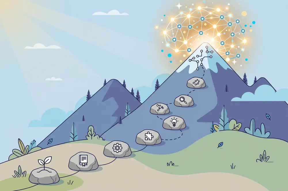
Open any "learn AI" thread online and you will find fifty contradictory roadmaps. Learn calculus first. No — learn Python first. No — just fine-tune a language model and skip the theory. Each advisor is describing the path that worked for them, in their field, with their background. The confusion is not a sign that you are behind; it is a sign that "AI" is not one subject. It is a continent with several countries, and the right route depends on where you want to end up.

Consider three researchers. Sara is an MS student in computer science who wants to publish in natural language processing. Bilal is an electrical engineer doing a PhD on fault detection in power systems, and his data is sensor readings in tables. Dr. Hina is a public-health researcher who wants to use machine learning on survey data but has never programmed. All three need "AI," but Sara needs transformers and large-scale training, Bilal needs time-series models and careful evaluation, and Hina needs basic Python and classical models she can explain to a medical audience. One roadmap cannot serve all three — but one map can, because the map shows every region and lets each traveler pick a route.

This chapter builds that map. By the end, you will know the major territories of AI, the order in which to visit them, what you can skip, and which route matches your research.

1.2 The five territories

Everything you need to learn fits into five territories. Think of them as layers: each layer rests on the one below it.

Territory 1: Mathematics. Linear algebra, calculus, and probability. This is the language AI is written in. You do not need a mathematics degree — you need working intuition, the ability to read an equation in a paper and translate it into an idea. Chapter 2 covers exactly how much, and no more.

Territory 2: Programming. Python, plus its three workhorse libraries: NumPy for numbers, pandas for tables, Matplotlib for plots. Nearly all AI research code lives in this ecosystem. Chapter 3 takes you from zero to useful.

Territory 3: Classical machine learning. Regression, classification, clustering, decision trees, support vector machines, and the discipline around them: train-test splits, cross-validation, overfitting, evaluation metrics. This is the territory most beginners skip, rushing to deep learning — and it is the territory that makes you dangerous, because most real research problems are solved here. Chapter 4 walks you through a complete project.

Territory 4: Deep learning. Neural networks, backpropagation, convolutional networks for images, transformers for language. Powerful, data-hungry, and easier to misuse than classical methods. Chapter 5 builds it step by step.

Territory 5: Specialization. Computer vision, natural language processing, or tabular/time-series data — plus the research skills that sit on top: reading papers, designing experiments, writing up results. Chapters 6 through 11 live here.

Notice the dependency order: you cannot do Territory 4 well without Territories 1–3, and you cannot do Territory 5 without 4 (or, for tabular researchers, sometimes 3 alone is enough — more on that in Chapter 6).

1.3 The 80/20 of AI learning

A useful rule: 20% of the material explains 80% of what you see in practice. The high-leverage 20% looks like this:

• Math: vectors, matrices, dot products, derivatives, the chain rule, gradients, probability distributions, Bayes' theorem, expected value. That is most of it.
• Programming: loops, functions, lists, dictionaries, NumPy arrays, pandas DataFrames, one plotting library.
• Machine learning: train/test split, linear and logistic regression, decision trees and random forests, k-means, cross-validation, precision/recall, overfitting.
• Deep learning: what a neuron computes, what a loss function measures, how gradient descent updates weights, what backpropagation is (intuitively), CNNs for images, transformers for sequences.
• Practice: one end-to-end project beats ten half-finished tutorials.

The remaining 80% — advanced optimization theory, custom CUDA kernels, the latest architecture variants — matters only after you have the 20% working. Beginners invert this: they study the exotic 80% and cannot build the basic 20%. Do not be that learner.

1.4 What you can skip (for now)

Permission to skip is as valuable as a study plan. For your first six months, you can safely postpone:

• Advanced calculus (multivariable proofs, real analysis). You need gradients, not theorems.
• Building models from raw C++ or CUDA. Use PyTorch or TensorFlow; the frameworks handle the hardware.
• The newest paper on arXiv every week. Fundamentals first; the frontier will still be there.
• MLOps and deployment (Docker, cloud serving, model monitoring). Important for industry, not for your first year of learning or your thesis experiments.
• Reinforcement learning, unless your research is in robotics or games. It is a wonderful field and a terrible starting point.
• Statistics at the measure-theory level. Applied probability is enough.

Skipping is not quitting. It is sequencing. Write these on a "later" list and return when a real problem demands them.

1.5 Three learner scenarios

Scenario A: Sara, the CS graduate. Sara finished a bachelor's in computer science. She knows Python and data structures but her math is rusty and she has never trained a model. Her route: spend three weeks refreshing linear algebra and calculus (Chapter 2, targeted sections), one week on NumPy/pandas (Chapter 3, fast track), then move straight into Chapters 4 and 5. Her 12-month goal: reproduce a published NLP result and extend it. Total ramp to productive research: about four months.

Scenario B: Bilal, the engineer. Bilal's PhD is about detecting faults from sensor data. He is strong in math and MATLAB but has never used Python. His route: skip most of Chapter 2 (he already has the math), spend two focused weeks converting his MATLAB thinking to Python/NumPy (Chapter 3), then master classical ML deeply (Chapter 4, plus extra time on time-series evaluation). He may never need deep learning — tree-based models on tabular sensor features might beat neural networks on his data, and Chapter 6 will help him decide. His 12-month goal: a baseline model and a careful evaluation methodology for his thesis.

Scenario C: Dr. Hina, the non-programmer. Hina is a public-health researcher with survey data and no coding background. Her route: Chapters 2 and 3 slowly, with emphasis on probability (her field already thinks statistically) and pandas (her data is tables). Then Chapter 4 only — logistic regression and random forests, which she can explain to clinicians. She does not need deep learning at all. Her 12-month goal: one analyzed dataset, one conference paper. Her biggest risk is not math; it is quitting Python in week three. Her plan needs small daily wins, which Chapter 3 provides.

Find yourself in one of these scenarios, or blend them. Your route is the chapters in order, with the emphasis each scenario suggests.

1.6 Your first-week action plan

Do not start by buying five courses. Start with one week of orientation:

1. Day 1–2: Read this chapter and Chapter 2's opening. Write down your research question in one sentence and which territory it lives in.
2. Day 3: Install Python (the Anaconda distribution is the simplest path for beginners) and run your first notebook. Type, do not copy-paste, the five-line NumPy example in Chapter 3.
3. Day 4–5: Work through the first half of Chapter 2's linear algebra section with a notebook open beside you. Every new concept gets one tiny code experiment.
4. Day 6: Pick your scenario (A, B, or C) and write your personal 12-month outline using Chapter 12 as a template — in pencil, expecting revisions.
5. Day 7: Rest. Then find one community from Chapter 9 and introduce yourself. Learning alone is slower; fix that in week one.

The whole journey is visible from here: math and Python in months 1–3, classical ML in months 3–5, deep learning in months 5–8, specialization and papers in months 8–12. The chapters ahead fill in every step. Turn the page and start with the only math you actually need.

1.7 Two mental models that carry you through the whole book

Before the study plans begin, adopt two mental models. They will make every later chapter easier, because nearly everything in AI is a variation on them.

Mental model 1: every supervised model is a function. Write it as ŷ = f(x): the model takes inputs x (house features, an image, a sentence) and produces an output ŷ (a price, a label, a reply). "Learning" means searching through possible functions to find one that maps inputs to correct outputs on data you have — and, the hard part, on data you have not seen. When a new algorithm confuses you, ask three questions: what is x here, what is ŷ, and how does this algorithm search for f? Linear regression searches among straight-line functions. A neural network searches among flexible layered functions. A decision tree searches among staircase functions. Different search spaces, same game. This single lens demystifies most of Chapters 4 and 5 in advance, and it gives you a fixed vocabulary for reading papers: every method section is, at bottom, a proposal for a better f or a better search.

Mental model 2: results come from a triangle — data, model, evaluation. Beginners obsess over the model corner ("which algorithm should I use?") and neglect the other two. Experienced practitioners know the triangle's secret: data quality usually beats model choice, and evaluation design determines whether your conclusions are even true. A mediocre model on great data with honest evaluation beats a fancy model on messy data with leaky evaluation — every time. Whenever you are stuck, check the triangle in order: is my data right? Is my evaluation honest? Only then: is my model appropriate? This ordering will save you months across Chapters 4, 5, 8, and 11, because most "model problems" turn out to be data or evaluation problems in disguise.

What success looks like at each stage. After the foundations (Chapters 2–3), you can read a paper's methods section and translate its math into ideas. After classical ML (Chapter 4), you can build an honest baseline for any tabular problem. After deep learning and specialization (Chapters 5–6), you can reproduce published results in your track. After the research chapters (7–11), you can design experiments that produce defensible, publishable conclusions. If you ever feel lost, locate yourself on this ladder — it tells you exactly which chapter to revisit.

How to use this book: three reading paths. Cover to cover is the default — chapters are sequenced by dependency. Fast track is for readers with background: take the Chapter 1 scenario test, skim chapters you know (but attempt every milestone), and slow down where you are weak. Reference mode is for later: when a project demands it, return to single chapters — Chapter 7 when the literature review starts, Chapter 11 when experiments begin. Whichever path you take, do the end-of-book exercises: they are designed as the building blocks Chapter 10 insists on.

For your research: Before you learn anything else, write your thesis or publication question in one sentence, then map it to a territory. "Predicting crop yield from satellite images" is computer vision (Territory 5, vision track). "Classifying customer complaints by topic" is NLP (Territory 5, language track). "Predicting student dropout from records" is tabular ML (Territory 3 may be enough). This single mapping decides which chapters deserve your deepest effort and which you can skim — it is the highest-leverage decision in this book.

Key takeaways: - AI is five territories in dependency order: math → programming → classical ML → deep learning → specialization. - Learn the 20% that explains 80%: vectors, gradients, probability, Python basics, train/test discipline, and what a neural network computes. - Skip advanced calculus, CUDA, MLOps, and reinforcement learning for now — sequence them later. - Match your route to your background: the CS graduate, the engineer, and the non-programmer take different paths through the same map. - Your first week: orient, install Python, touch linear algebra, draft your 12-month outline, join one community.

---

Chapter 2: Math Foundations: Only What You Actually Need

2.1 The math myth

Ask a beginner what blocks them from learning AI and the most common answer is mathematics. Somewhere they absorbed the idea that you need a mathematics degree — real analysis, measure theory, advanced linear algebra — before you may touch a neural network. This is false, and it is one of the most expensive falsehoods in AI education, because it keeps capable researchers studying math for a year instead of building models in a month.

Here is the honest version. You need working intuition for three areas: linear algebra, calculus, and probability. Working intuition means: when a paper writes an equation, you can translate it into an idea ("this is measuring the distance between prediction and truth"), and when your code needs it, you can compute it with NumPy rather than by hand. You do not need to prove theorems. You do not need to solve integrals on paper. The computer does arithmetic; you supply understanding.

There is also a strategy question: when to learn the math. The winning strategy is just-in-time learning. Learn a concept the week before you need it, in the context of needing it. Gradients make sense when you are about to train a model and need to know why weights change. Bayes' theorem makes sense when you are building a classifier and need to reason about uncertainty. Math learned just-in-time sticks; math learned "just in case" evaporates.

2.2 Linear algebra: the language of data

Nearly every object in machine learning is a vector or a matrix. A dataset with 1,000 houses and 10 features per house is a 1,000 × 10 matrix. A single house is a vector of 10 numbers. A linear model's weights are a vector. Images are matrices (or 3D arrays). Once you see the world this way, half of ML notation becomes readable.

The minimum set:

• Vectors and scalars. A vector is an ordered list of numbers, like [1500, 3, 2] for a house (square feet, bedrooms, bathrooms). A scalar is a single number. Vector addition and scalar multiplication are exactly what they sound like.
• Dot products. The dot product of two vectors multiplies matching entries and adds them up: [1, 2, 3] · [4, 5, 6] = 1×4 + 2×5 + 3×6 = 32. This single operation is everywhere: a linear model prediction is just a dot product of weights and features, plus a bias. When you see wᵀx in a paper, read it as "dot product of weights and input" — a weighted sum.
• Matrices and matrix multiplication. A matrix is a table of numbers. Multiplying matrices composes linear transformations. The key intuition: a matrix transforms vectors — it can rotate, stretch, or project them. A neural network layer is a matrix multiplication followed by a nonlinearity. That sentence, understood deeply, explains most of deep learning's machinery.
• Norms. A norm measures a vector's size. The L2 norm (Euclidean length) appears in regularization and distance metrics. When a paper says "minimize the norm of the weights," it means "keep the model simple."
• Eigenvalues and eigenvectors (intuition only). Some vectors keep their direction when a matrix transforms them, only stretching or shrinking — those are eigenvectors, and the stretch factor is the eigenvalue. You need this intuition for one reason: principal component analysis (PCA), a dimensionality-reduction technique, is built on it. Understand the sentence above and you understand what PCA is doing.

How to learn it: watch a visual linear algebra series (the 3Blue1Brown "Essence of Linear Algebra" series is the standard recommendation for good reason), and after each video, reproduce the idea in NumPy. Ten lines of NumPy teach more than ten pages of definitions:

import numpy as np

w = np.array([0.5, -1.2, 0.8])   # weights
x = np.array([1500, 3, 2])       # one house: sqft, bedrooms, bathrooms
prediction = w.dot(x) + 10.0     # linear model: weighted sum + bias
print(prediction)                # 758.0

That is a linear model. Everything else in this section is vocabulary for describing variations of this idea.

2.3 Calculus: the language of learning

If linear algebra is the language of data, calculus is the language of learning. Models learn by adjusting their weights to reduce error, and calculus tells them which direction to adjust. The entire concept reduces to one idea: the derivative.

A derivative measures how much a function's output changes when you nudge its input. If the error goes down when you increase a weight, the derivative is negative, and the learning algorithm increases that weight. That is gradient descent, the engine of modern AI, in one paragraph. Chapter 5 and the gradient-descent literature build on this, but the intuition is already complete.

The minimum set:

• Derivatives of basic functions. Know that the derivative of x² is 2x, of eˣ is eˣ, and that constants vanish. You will look up the rest.
• The chain rule. If y depends on u and u depends on x, then dy/dx = dy/du × du/dx. This is the single most important calculus rule in AI because neural networks are chains of functions — the chain rule is literally how backpropagation computes gradients through layers. Understand it once, intuitively: "to know how the output changes with an early weight, multiply the sensitivities along the path."
• Partial derivatives and gradients. A model has thousands of weights. The partial derivative says how the error changes when you nudge one weight holding others fixed. Collect all partial derivatives into a vector and you have the gradient: the direction of steepest increase of the error. Gradient descent steps in the opposite direction. When a paper writes ∇L (del L), read "the gradient of the loss" — an arrow pointing uphill, which the algorithm walks downhill away from.
• A worked example. Take the simplest loss, mean squared error for one prediction: L = (y − ŷ)², where ŷ = wx. The derivative with respect to w is dL/dw = −2(y − ŷ)x. Read it: the weight update is proportional to the error (y − ŷ) and the input x. Big error, big update. Wrong sign, push the other way. You now understand the update rule of linear regression at the level that matters.

What to skip: integration techniques, multivariable proofs, differential equations. If a paper needs them, learn that specific piece then.

2.4 Probability and statistics: the language of uncertainty

Machine learning is applied probability wearing a practical jacket. Data is noisy, the future is uncertain, and models output probabilities, not certainties. Researchers from statistics-heavy fields (medicine, economics, agriculture) often find this the easiest territory — and everyone else should treat it as equally important as calculus.

The minimum set:

• Probability basics. An event's probability is between 0 and 1. The probability of A and B (for independent events) multiplies; of A or B adds (minus the overlap). A surprising amount of ML reasoning is just careful application of these rules.
• Distributions. The normal (bell curve) distribution describes measurement noise; the Bernoulli describes yes/no outcomes; the categorical describes multi-class outcomes. Know what each looks like and when it appears. When a paper says "assume Gaussian noise," it means "assume bell-curve-shaped errors" — a modeling choice, not a law of nature.
• Bayes' theorem. P(A|B) = P(B|A) × P(A) / P(B). In words: update your belief about A after seeing evidence B. This is the logic of spam filters, medical diagnosis models, and Bayesian ML generally. Work one numerical example by hand — a disease test with 99% accuracy on a rare disease — and you will never forget why base rates matter. (With a 1-in-1,000 disease and a 1% false-positive rate, most positive tests are false alarms. That single insight will make you a more careful evaluator of classifiers forever.)
• Expected value. The average outcome weighted by probability. Loss functions are usually expected values: "on average, over all data, how wrong are we?" When a paper writes E[·], read "the average of."
• Hypothesis testing basics. p-values, confidence intervals, and the idea of statistical significance. You need these to read experimental sections honestly and to avoid fooling yourself with a lucky split. Know that "significant" has a technical meaning (unlikely under the null hypothesis) distinct from "important."
• Maximum likelihood intuition. Many models are trained by asking: "which parameters make the observed data most probable?" That is maximum likelihood estimation. Logistic regression, for example, is trained this way. One sentence of intuition covers dozens of papers' training sections.

How to learn it: simulate. Probability learned through simulation is probability understood. Flip 10,000 virtual coins in NumPy, plot the results, watch the bell curve emerge:

import numpy as np
import matplotlib.pyplot as plt

flips = np.random.randint(0, 2, size=10000)   # 10,000 fair coin flips
heads_counts = [np.random.randint(0, 2, size=100).sum() for _ in range(1000)]
plt.hist(heads_counts, bins=20)
plt.title("Heads in 100 flips, repeated 1000 times")
plt.xlabel("Number of heads")
plt.show()

Run it. The histogram will be bell-shaped around 50. You have just seen the central limit theorem instead of memorizing it.

2.5 The just-in-time study plan

Here is a concrete six-week plan at about five hours per week. Each week pairs theory with immediate coding, because math without code is trivia.

• Weeks 1–2: Linear algebra. Visual lessons on vectors, dot products, matrices, and transformations. After each lesson, reproduce it in NumPy: create the vectors, do the multiplication, plot a transformation of a grid of points. End of week 2 test: explain in your own words what wᵀx + b computes and implement linear regression's prediction step from scratch.
• Weeks 3–4: Calculus. Derivatives of basic functions, the chain rule (spend real time here — draw the chain as a diagram), partial derivatives, gradients. Code gradient descent for a one-parameter problem by hand: start with a wrong weight, compute the gradient, step downhill, watch the loss fall. End of week 4 test: derive the gradient of mean squared error and implement it.
• Weeks 5–6: Probability. Distributions via simulation, Bayes' theorem with the disease-test example, expected value, maximum likelihood intuition. Code the coin-flip simulation and a tiny Naive Bayes spam classifier on toy data. End of week 6 test: explain why accuracy can mislead on imbalanced data, using a numerical example.

If you already know some area, compress or skip its weeks — Bilal the engineer, from Chapter 1, might do this whole plan in ten days as a refresher. If an area fights you, extend it by a week rather than pushing through confused; confusion compounds.

2.6 Math you will meet later (and can ignore now)

As you read papers you will encounter heavier machinery: information theory (entropy, KL divergence), optimization theory (convexity, Lagrangians), linear algebra beyond the basics (SVD, matrix calculus), and Bayesian nonparametrics. Treat each as a just-in-time topic. When a paper you need uses KL divergence, spend an afternoon learning exactly KL divergence — its definition, its intuition ("how surprised one distribution is by another"), and one coded example. You will learn it ten times faster with a concrete reason than you would from a textbook chapter read "in preparation."

For your research: List the three most important papers for your thesis topic. Skim their methods sections and circle every mathematical object you cannot explain in one sentence — each circle is a just-in-time learning task. Most students find only five to ten distinct concepts, not the hundreds they feared. Work through them one per week, each with a small coded example, and within two months you will read your subfield's papers fluently. Keep the list; it becomes the math appendix of your literature review.

Key takeaways: - You need working intuition for three areas only: linear algebra, calculus, probability — not a math degree. - Linear algebra is the language of data (vectors, matrices, dot products); calculus is the language of learning (derivatives, chain rule, gradients); probability is the language of uncertainty (distributions, Bayes, expected value). - Learn just-in-time: study a concept the week you need it, paired with a small coding experiment. - The chain rule and the gradient are the two ideas that unlock backpropagation and modern training — invest in them. - Simulate probability instead of memorizing it; reproduce linear algebra in NumPy instead of reading definitions. - Six weeks at five hours per week covers the minimum viable math; compress what you know, extend what resists.

---

Chapter 3: Programming Foundations: Python from Zero

3.1 Why Python, and why it is enough

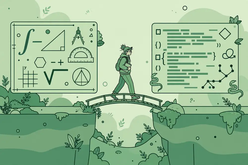
Every major AI library — scikit-learn, PyTorch, TensorFlow, Hugging Face Transformers — speaks Python. Research code, tutorials, and paper implementations are published in Python. This is not a technical judgment about the "best" language; it is a network effect you should simply join. Learning Python gives you immediate access to the entire ecosystem, and for research purposes Python is not a stepping stone to something else — it is the destination.

If you already program in another language (MATLAB, R, Java, C++), this chapter is a two-week conversion course: same ideas, new syntax, plus the three libraries below. If you have never programmed, this chapter is a six-week foundation. Both paths end at the same place: you can load data, manipulate it, plot it, and train a model.

A note on setup, because setup kills more beginners than syntax does. Install the Anaconda distribution of Python, which bundles Python with NumPy, pandas, Matplotlib, Jupyter, and scikit-learn in one installer. Open Jupyter Notebook, create a new notebook, and type your first cell. Do not spend a week choosing editors, configuring environments, or reading about virtual environments — those matter later, and Chapter 11 covers them. Your only goal this week is a running notebook.

3.2 Core Python in one pass

You need a working subset of Python, not the whole language. Here it is, with the smallest possible complete example of each idea. Type every example yourself — typing is thinking.

Variables and types. A variable is a named box holding a value. Python has integers, floats, strings, and booleans, and you rarely need to think about which is which:

house_price = 250000      # int
area = 1500.5             # float
city = "Karachi"          # string
is_sold = True            # boolean

Lists and dictionaries. A list is an ordered collection; a dictionary maps keys to values. Together they represent nearly all structured data you will touch before pandas takes over:

prices = [250000, 320000, 180000]          # list of house prices
house = {"area": 1500, "bedrooms": 3, "city": "Karachi"}  # dict
print(prices[0])        # 250000 (lists start at 0)
print(house["bedrooms"]) # 3

Loops and conditions. A for loop repeats an action; an if chooses between actions. Most data work is loops plus conditions, even when libraries hide them:

for price in prices:
    if price > 200000:
        print(price, "is expensive")

Functions. A function packages reusable logic with a name. Write functions early and often — a notebook full of copy-pasted cells is where bugs hide:

def predict_price(area, price_per_sqft=150):
    """Predict price from area. price_per_sqft has a default value."""
    return area * price_per_sqft

print(predict_price(1500))        # 225000
print(predict_price(1500, 200))   # 300000

List comprehensions (one step beyond basics, worth learning immediately because ML code is full of them):

areas = [1200, 1500, 1800]
predictions = [predict_price(a) for a in areas]  # apply to each

That is the core. Strings, files, classes, decorators, and the rest can wait until a project demands them.

3.3 NumPy: thinking in arrays

NumPy replaces Python loops with fast array operations, and — more importantly — it lets you think in vectors and matrices, which is exactly the linear algebra of Chapter 2 made executable. The central rule: never loop over numbers when NumPy can operate on the whole array at once. This style is called vectorization, and it is both faster and more readable.

import numpy as np

# Chapter 2's linear model, now in NumPy
w = np.array([0.5, -1.2, 0.8])
X = np.array([[1500, 3, 2],
              [1200, 2, 1],
              [2000, 4, 3]])      # 3 houses, 3 features each
predictions = X.dot(w) + 10.0     # one line, all three houses
print(predictions)

# Statistics in one line each
print("Mean:", X[:, 0].mean())    # average of column 0 (area)
print("Std: ", X[:, 0].std())     # spread of areas

# Broadcasting: subtract the mean from every row at once
centered = X - X.mean(axis=0)

Three ideas carry 90% of NumPy: array creation (np.array, np.zeros, np.arange, np.random.randn), indexing (X[0], X[:, 1], boolean masks like X[X[:, 0] > 1500]), and vectorized operations (arithmetic, .dot(), .mean(), .sum()). Practice these on small arrays until they feel like arithmetic. A common beginner error is shape mismatch — when NumPy complains, print .shape of each array; the bug is always a wrong dimension, and checking shapes is the professional debugging habit.

3.4 pandas: thinking in tables

Real data arrives as tables: CSV files, spreadsheets, database exports. pandas' DataFrame is a table with superpowers — load, filter, group, summarize, and clean in a few lines. If your research data is tabular (surveys, sensor logs, financial records), pandas is the tool you will use daily.

import pandas as pd

# Load and inspect: the first three lines of every data analysis
df = pd.read_csv("houses.csv")
print(df.head())        # first 5 rows
print(df.describe())    # means, mins, maxes per column
print(df.isnull().sum())# missing values per column — always check this

# Filter, select, group: the verbs of data work
expensive = df[df["price"] > 300000]          # rows matching a condition
avg_by_city = df.groupby("city")["price"].mean()  # average price per city

# Handle a missing value and create a feature
df["area"] = df["area"].fillna(df["area"].median())
df["price_per_sqft"] = df["price"] / df["area"]   # feature engineering

Learn these verbs first: read_csv, head, describe, isnull, boolean filtering, groupby, fillna, dropna, merge. Everything else — pivot tables, multi-indexes, time-series resampling — is just-in-time material. One warning: pandas has many ways to do the same thing, which confuses beginners. Pick the simple verbs above and ignore the rest until needed.

3.5 Matplotlib: thinking in pictures

You cannot debug what you cannot see. Plot early, plot often: distributions of features, predictions versus truth, loss curves during training. Matplotlib is verbose but universal; learn the basic pattern and reuse it forever:

import matplotlib.pyplot as plt

plt.scatter(df["area"], df["price"])   # one plot: does price rise with area?
plt.xlabel("Area (sq ft)")
plt.ylabel("Price")
plt.title("House price vs. area")
plt.show()

The pattern is always: create data, call a plot function (plot, scatter, hist, bar), label axes, show. Histograms (plt.hist) reveal distributions and outliers; scatter plots reveal relationships; line plots reveal trends over time or training iterations. When a model misbehaves in Chapter 4, your first move will be a plot, not a hyperparameter.

3.6 Notebooks versus scripts, and the reproducibility habit

Jupyter notebooks are wonderful for exploration and terrible for reproducibility — cells can run out of order, leaving hidden state that makes results unrepeatable. Adopt this discipline from day one:

1. Explore in notebooks, keep in scripts. Once an analysis works, move the important logic into a .py file with functions.
2. Restart and run all before trusting any notebook result. If the numbers change, you had hidden state.
3. Set random seeds (np.random.seed(42)) so your results are repeatable.
4. One notebook, one question. A notebook titled "analysis_final_v7_REAL.ipynb" is a cry for help; split by question instead.

These habits feel slow now and save weeks later — especially when a reviewer asks you to reproduce a result six months after you made it.

3.7 The six-week (or two-week) plan

From zero (six weeks, ~5 hrs/week): Weeks 1–2: core Python — variables through functions, plus fifty tiny exercises (write a function, break it, fix it). Weeks 3–4: NumPy — redo every Chapter 2 linear algebra example as code; vectorize three loop-based programs. Weeks 5–6: pandas and Matplotlib on a real CSV dataset (any public dataset with at least 1,000 rows): load it, clean it, answer five questions about it with grouped summaries and plots, and write up the answers in a one-page report. The report matters — it practices the communication researchers need.

Converting from another language (two weeks): Week 1: Python syntax differences that bite converts — zero-based indexing, indentation instead of braces, None instead of null, list comprehensions, and the fact that a = b on arrays copies the reference, not the data (use .copy()). Week 2: NumPy as "MATLAB with different syntax," pandas as "better data frames," and the notebook workflow. Your test: reimplement one analysis you previously did in MATLAB or R, end to end, in Python.

The scenario check: Dr. Hina from Chapter 1 is the from-zero learner — her success criterion is not elegance but persistence: code a little every day, and by week six she can load her survey data and plot it. Sara the CS graduate does the two-week conversion. Bilal does the two-week conversion plus a NumPy deep-dive since his sensor work is array-heavy.

3.8 Debugging: the skill nobody teaches

You will spend more time debugging than writing new code — every programmer does, and researchers debugging experiments doubly so. Debugging is a learnable skill with a method, and learning it now pays off in every later chapter.

Read the error bottom-up. When Python fails, it prints a traceback: a stack of function calls ending in the actual error. Beginners read top-down and panic; professionals read the last line first — it names the error, e.g. NameError: name 'df' is not defined — then find the line of your code it points to. Eighty percent of bugs are identified right there: a typo, a variable used before it was created (often from running notebook cells out of order — Chapter 3's restart-and-run-all rule prevents this class entirely).

Learn the usual suspects. You will meet these weekly, so memorize the fixes: NameError (typo or out-of-order cells); TypeError (wrong kind of object, like adding a string to a number — check what each variable actually is); IndentationError (mixed tabs and spaces — set your editor to insert spaces); IndexError (index out of range — remember zero-based indexing, and that a length-5 list has no index 5); KeyError (misspelled dictionary key or DataFrame column — print df.columns to see the real names); NumPy ValueError about shapes not aligning (print .shape on both arrays — the bug is always a dimension); and pandas' infamous SettingWithCopyWarning (you modified a slice of a DataFrame instead of the DataFrame — fix it with .loc indexing or an explicit .copy()).

Shrink the bug. Reproduce the error in the smallest possible script — five lines if you can. Half the time, shrinking reveals the cause; the other half, it produces something you can actually ask about in a community (Chapter 9), where a minimal example gets answers and a 300-line dump gets ignored.

Explain it out loud. The "rubber duck" method — describing your code line by line to an inanimate object or a patient friend — works because explaining forces you to state assumptions, and the bug is always a wrong assumption. "This variable should be a DataFrame here because..." — stop, check: is it? Print its type. The number of bugs caught by one well-placed print(type(x)) is legendary.

Mindset and recovery. The computer executes exactly what you wrote, not what you meant. When a bug feels "impossible," that feeling marks the wrong assumption — get curious instead of frustrated. Keep a debugging checklist taped to your wall: restart kernel and run all; check shapes and types; shrink to minimal; search the exact error message. And take breaks: a fifteen-minute walk solves more bugs than a third hour of staring, because fresh eyes re-read assumptions instead of re-reading code.

For your research: Your first research-grade Python artifact is a "data diary" notebook for your own dataset: load it, document every column in markdown cells, plot every distribution, count missing values, and write down three observations and three questions. This single notebook becomes the methods section's data description later, and the questions become your first experiments. Researchers who skip this step build models on data they do not understand; researchers who do it catch the data errors that would have invalidated their results.

Key takeaways: - Python is the destination, not a stepping stone: the whole AI ecosystem speaks it. - Core Python subset: variables, lists, dicts, loops, conditions, functions, comprehensions. - NumPy: think in arrays; vectorize instead of looping; check .shape when debugging. - pandas verbs: load, inspect, filter, group, clean — enough for most research data work. - Matplotlib pattern: plot, label, show — plot early and often to see what your data and models do. - Explore in notebooks, keep logic in scripts; restart-and-run-all; set random seeds. - From zero: six weeks. Converting: two weeks. Daily practice beats weekend marathons.

---

Chapter 4: Your First Machine Learning Project, Step by Step

4.1 Why one project beats ten tutorials

Tutorials teach you to follow; projects teach you to decide. Every tutorial hands you clean data, a chosen model, and the right metric. Real projects — including thesis research — hand you a messy question and make you choose everything. The gap between "I completed the course" and "I can do machine learning" is exactly one end-to-end project wide. This chapter walks you through that project, slowly, so your second one is independent.

We will predict house prices from house features — the classic regression problem. It is simple enough to complete in a weekend and rich enough to contain every step of real ML work. Follow along in a notebook, typing every line.

4.2 Step 1: Frame the problem

Before touching data, answer three questions in writing:

1. What exactly am I predicting? The sale price of a house, a continuous number. This is regression (predicting a number), not classification (predicting a category). The problem type decides everything downstream: the models, the loss, the metrics.
2. What are my inputs? Features like area, bedrooms, bathrooms, location. Write down what you have, not what you wish you had.
3. How will I know I succeeded? Pick a metric now: mean absolute error (MAE) — "on average, my prediction is off by this many dollars." A metric chosen after seeing results is a metric chosen to flatter you.

Write a one-paragraph problem statement. Researchers skip this and pay for it later when their experiments answer a different question than their thesis asks.

4.3 Step 2: Get and explore the data

Load the data and interrogate it before modeling. Use your Chapter 3 data diary: shapes, missing values, distributions, and the target's range. Two plots are mandatory: a histogram of the target (is it skewed? are there absurd outliers?) and scatter plots of each feature against the target (is there any visible relationship?). If no feature visibly relates to the target, no model will find magic — go get better features.

Split the data before any modeling, and understand why: the test set is your unbiased judge. If the model sees it during training, your evaluation is fiction. The standard split:

from sklearn.model_selection import train_test_split

X_train, X_test, y_train, y_test = train_test_split(
    X, y, test_size=0.2, random_state=42
)

Eighty percent to learn from, twenty percent locked away for final judgment. The random_state makes the split reproducible.

4.4 Step 3: Train a baseline (the most important step)

Train the simplest reasonable model first — linear regression — and record its error. This baseline is your anchor: every fancier model must beat it to justify its complexity, and half the time, it will not. Researchers who skip baselines publish "improvements" over nothing.

from sklearn.linear_model import LinearRegression
from sklearn.metrics import mean_absolute_error, mean_squared_error

model = LinearRegression()
model.fit(X_train, y_train)          # learn weights from training data

pred = model.predict(X_test)         # predict on unseen data
print("MAE:", mean_absolute_error(y_test, pred))
print("RMSE:", mean_squared_error(y_test, pred) ** 0.5)

Read the MAE in plain language: "on unseen houses, I am off by $X on average." Is that good? Compare it to a dumb baseline: predicting the mean price for every house. If your model barely beats the mean, your features carry little signal — a data problem, not a model problem.

4.5 Step 4: Try a stronger model and compare honestly

Now try a random forest — an ensemble of decision trees that handles nonlinearity and needs little tuning:

from sklearn.ensemble import RandomForestRegressor

rf = RandomForestRegressor(n_estimators=100, random_state=42)
rf.fit(X_train, y_train)
pred_rf = rf.predict(X_test)
print("RF MAE:", mean_absolute_error(y_test, pred_rf))

Compare on the same test set with the same metric. If the forest wins clearly, you have evidence the relationship is nonlinear. If it barely wins, prefer the simpler linear model — simpler models are easier to explain, debug, and defend in a thesis. Also inspect which features matter:

import pandas as pd
importances = pd.Series(rf.feature_importances_, index=X.columns)
print(importances.sort_values(ascending=False))

Feature importances turn the model from a black box into a story: "area and location drive price; bedrooms add little." That story is what your thesis committee actually wants.

4.6 Step 5: Validate properly and avoid fooling yourself

One train/test split can be lucky. Cross-validation repeats the split several times and averages the result:

from sklearn.model_selection import cross_val_score

scores = cross_val_score(rf, X, y, cv=5, scoring="neg_mean_absolute_error")
print("CV MAE:", -scores.mean(), "+/-", scores.std())

If cross-validation error is much worse than your single-split error, your first split was lucky — trust the cross-validated number. Two more honesty rules: never tune hyperparameters on the test set (tune on a validation split or via cross-validation, then evaluate once on the test set), and never let information from the test set leak into training — for example, computing feature scaling statistics on the full dataset before splitting. Leakage is the most common way beginners report fantastic, fictional results.

4.7 Step 6: Iterate with a hypothesis, not randomly

Improvement comes from hypotheses, not from trying forty models. Each iteration should be a small experiment: "I believe adding price-per-square-foot as a feature will help because..." → implement → measure → keep or discard. Log every experiment: date, change, MAE, note. A simple table in your notebook is enough. After ten logged experiments you will notice something: your judgment about what helps improves faster than any single model's score. That judgment is the actual skill of machine learning.

Know when to stop: when additional experiments move the metric by less than the noise between cross-validation folds, you are done. Diminishing returns are a signal to write up, not to tune harder.

4.8 A weekend project plan

• Saturday morning (3 hrs): Frame the problem in writing; load and explore data; write the data diary.
• Saturday afternoon (3 hrs): Train/test split; linear regression baseline; dumb-mean comparison; first plots of predictions vs. truth.
• Sunday morning (3 hrs): Random forest; feature importances; cross-validation; fix one data issue you spotted (missing values, an outlier).
• Sunday afternoon (2 hrs): Three hypothesis-driven iterations, logged; write a one-page report with the problem, method, results table, and what you would try next.

Eleven hours, one complete project, one report. Repeat with a new dataset (a classification problem next — the classic Iris flower dataset is ideal for your second project) and you will have the core ML loop in muscle memory.

4.9 A second worked example: classification in thirty minutes

Regression predicts numbers; classification predicts categories — and most research questions are classification: disease or healthy, churn or stay, topic A, B, or C. The workflow is identical to Sections 4.2–4.7; only the model and the metrics change. Here is the compressed version on the classic Iris flower dataset (150 flowers, 4 measurements each, 3 species):

from sklearn.datasets import load_iris
from sklearn.model_selection import train_test_split, cross_val_score
from sklearn.linear_model import LogisticRegression
from sklearn.metrics import confusion_matrix, classification_report

X, y = load_iris(return_X_y=True)
X_train, X_test, y_train, y_test = train_test_split(
    X, y, test_size=0.2, random_state=42, stratify=y
)

clf = LogisticRegression(max_iter=200)
clf.fit(X_train, y_train)
print("Accuracy:", clf.score(X_test, y_test))
print(confusion_matrix(y_test, clf.predict(X_test)))
print(classification_report(y_test, clf.predict(X_test)))

Three things to notice. First, stratify=y keeps class proportions identical in train and test splits — without it, a small test set might contain zero examples of a rare class, silently invalidating your evaluation. Make stratified splitting a reflex for every classification project. Second, the confusion matrix is the evaluation tool that matters most: rows are true classes, columns are predicted classes, and off-diagonal entries show exactly which mistakes the model makes. A model confusing two similar Iris species is telling you something about the data — perhaps those species genuinely overlap in these measurements — which is a scientific observation, not just an error. Always inspect the confusion matrix before the accuracy number.

Third, the classification report shows precision and recall per class, and this is where Chapter 2's disease-test intuition becomes practical. On imbalanced data — say 95% healthy patients, 5% sick — a model predicting "healthy" for everyone scores 95% accuracy while finding zero sick patients. Accuracy lies; precision ("of my alarms, how many were real?") and recall ("of the real cases, how many did I catch?") tell the truth. Choose which to optimize by the cost of errors: in disease screening, missing a case (low recall) harms more than a false alarm (low precision), so you optimize recall even at precision's expense. In spam filtering the costs reverse — users hate losing real email — so you optimize precision. This error-cost thinking turns metrics from numbers into decisions, and a paragraph of it belongs in every thesis's evaluation section: state your costs, then justify your metric.

Common classification mistakes (check yourself against this list on every project): tuning hyperparameters on the test set (Chapter 4's rule still applies); ignoring class imbalance (consider class weights or resampling, and always report per-class metrics); forgetting stratify in splits; leaking through preprocessing (fit scalers on training data only); and comparing models on different splits. Finish with cross-validation as in Section 4.6, and you own the complete classification loop.

Your turn this week: take the classification loop to a dataset of your own — ideally related to your research. Write the framing paragraph (Section 4.2), run the loop, and produce the one-page report: problem, method, confusion matrix, precision/recall with error-cost justification, and what you would try next. Two worked examples (regression and classification) plus one of your own means the ML loop is no longer something you read about — it is something you do.

4.10 The experiment log: your memory, externalized

Chapter 4 mentioned logging experiments; here is the concrete template. Keep it as a simple table — spreadsheet or markdown — with one row per experiment and these columns: Date | Code version | Change (one variable!) | Train metric | Validation metric | Test metric | Note. Example rows from the house-price project:

Date	Ver	Change	Val MAE	Note
Mon	a1f3	baseline linear regression	$28,400	first honest number
Tue	b2e9	+ price_per_sqft feature	$26,100	helps; keep
Wed	c4d2	random forest, 100 trees	$24,800	nonlinear signal exists
Thu	d7a1	RF, max_depth=5 (simpler)	$25,000	slight loss; keep depth open

Five rules make the log work: log before you forget (same day); one variable per row or the row is uninterpretable; always record the code version (a Git hash) so any row is reproducible; write the note as a decision ("keep"/"drop"/"investigate"), not just a number; and review weekly — patterns across rows ("every feature from location helps") become your domain intuition. When thesis-writing time comes, this log is your results section's first draft and your defense against "did you try X?" — because you can point to the row where you did. Bring the log to advisor meetings too: a table of dated, versioned experiments communicates progress more convincingly than any verbal summary, and it lets your advisor spot patterns you missed — "every time you add location features it helps; have you considered interaction terms?" That single comment can redirect a month of work productively.

For your research: Your thesis needs a baseline chapter, and this project is its prototype. Take your own dataset through these exact six steps and write it up as a technical report: problem framing, data description, baseline model, stronger model, honest evaluation with cross-validation, and an experiment log. Even if your final thesis uses deep learning, reviewers expect a simple baseline for comparison — the model you build this weekend is the "Model A" your future papers will cite as the thing you beat. Save the notebook; you will reuse its structure for every experiment you ever run.

Key takeaways: - Frame first: regression vs. classification, inputs, and success metric — in writing, before code. - Explore before modeling: distributions, missing values, and whether features visibly relate to the target. - Always train a simple baseline (and a dumb baseline) before anything fancy. - Compare models on the same test set with the same metric; prefer the simpler model when scores tie. - Use cross-validation; never tune on the test set; watch for data leakage. - Iterate with hypotheses and log every experiment; stop at diminishing returns. - One weekend, one dataset, one report: that is the unit of learning that builds real skill.

---

Chapter 5: Deep Learning, Step by Step

5.1 What actually changes when networks get deep

Classical machine learning, which you practiced in Chapter 4, works in two stages: a human designs features (price-per-square-foot, average sensor reading), and the model learns weights for those features. Deep learning collapses the two stages into one: the model learns the features itself, directly from raw data. Feed a network raw pixels and it discovers edges, then shapes, then objects — a hierarchy of features no human designed. This idea, called representation learning, is the entire reason deep learning exists, and it explains both its power and its appetite: discovering features from scratch requires far more data and computation than weighting human-designed ones.

A "deep" network simply means many layers stacked in sequence. Each layer transforms its input a little — the first layer might detect edges in an image, the next combines edges into textures, the next into parts, the next into objects. Depth is what lets the network build this hierarchy. The famous 2015 review by LeCun, Bengio, and Hinton [3] describes this hierarchy as the central idea of deep learning, and reading its first few pages is a worthwhile rite of passage once you finish this chapter.

But depth comes with costs you must respect. Deep models need large datasets (thousands to millions of examples), they train for hours or days rather than seconds, they overfit eagerly on small data, and they are harder to interpret — a real problem when your thesis committee asks why the model decided something. Chapter 6 will help you decide when deep learning is warranted; this chapter makes sure you understand it first.

5.2 The neuron, concretely

Strip away the mystique and a neuron is the linear model from Chapter 2 wearing one extra piece of clothing. It computes a weighted sum of its inputs, adds a bias, and passes the result through a nonlinear activation function:

z = w₁x₁ + w₂x₂ + ... + wₙxₙ + b     (weighted sum, as in Chapter 2)
a = activation(z)                      (nonlinearity — the new part)

Why the nonlinearity? Without it, stacking layers would be pointless: a stack of linear transformations is just one linear transformation, no matter how deep. The activation function — the most common is ReLU, which outputs max(0, z), passing positive values through and zeroing negatives — bends the straight lines into curves, letting the network approximate complex functions. Other activations you will meet: sigmoid (squashes to 0–1, used for binary outputs), tanh (squashes to −1 to 1), and softmax (turns a vector into probabilities summing to 1, used for multi-class outputs).

A layer is many neurons side by side, each with its own weights, all reading the same input. A network is layers in sequence: the outputs of one layer become the inputs of the next. The first layer sees raw features; the last layer produces the prediction; everything between is the "hidden" machinery learning representations.

5.3 Loss functions: telling the network what "wrong" means

A network learns by minimizing a loss function — a number measuring how wrong its predictions are. Choose the loss to match your problem:

• Mean squared error (MSE) for regression: average of squared differences between prediction and truth. Squaring punishes large errors heavily.
• Cross-entropy for classification: measures how far the predicted probabilities are from the true labels. When the model assigns 90% probability to the wrong class, cross-entropy is large; when it assigns 90% to the right class, it is small. Nearly all classification networks use it.

The loss is the compass: every training step asks "which weight changes reduce this number?" Understand the loss and you understand what the network is trying to do — which also tells you what it might do wrong. A model trained with MSE on house prices will happily sacrifice accuracy on cheap houses to nail expensive ones (large errors dominate), a bias you should know about before trusting it.

5.4 How networks learn: gradient descent and backpropagation

Training is a loop with three steps, repeated thousands of times:

1. Forward pass: feed training examples through the network, compute predictions and the loss.
2. Backward pass (backpropagation): compute the gradient of the loss with respect to every weight — how much each weight contributed to the error. This is the chain rule from Chapter 2, applied mechanically layer by layer, from output back to input. You never compute it by hand; the framework does. But you must understand what it computes: blame assignment. Each weight learns how guilty it is.
3. Update: nudge every weight a small step opposite the gradient: w = w − learning_rate × gradient. The learning rate controls step size — too large and training diverges wildly; too small and it crawls.

That is the whole algorithm. Everything else in deep learning training — optimizers like Adam (which adapt the step size per weight), learning rate schedules, batch normalization — is refinement of this loop. When training fails, diagnose it in these terms: is the loss even decreasing (learning rate problem)? Does training loss fall but validation loss rise (overfitting — Chapter 4's old enemy, back with more appetite)? Does the loss not move at all (vanishing gradients or a bug in the data pipeline)?

5.5 Your first network in code

Let us train a small neural network with PyTorch on a classification task. (Keras with TensorFlow is an equally fine choice — pick one framework and go deep rather than sampling both. This book uses PyTorch because most research code you will read is written in it.)

import torch
import torch.nn as nn

# A tiny network: input -> 64 neurons (ReLU) -> 32 neurons (ReLU) -> 1 output
model = nn.Sequential(
    nn.Linear(10, 64),   # 10 input features
    nn.ReLU(),
    nn.Linear(64, 32),
    nn.ReLU(),
    nn.Linear(32, 1),
    nn.Sigmoid()         # squash output to 0-1 for binary classification
)

criterion = nn.BCELoss()                    # binary cross-entropy loss
optimizer = torch.optim.Adam(model.parameters(), lr=0.001)

# The training loop: forward, backward, update — repeated
for epoch in range(100):
    optimizer.zero_grad()                   # clear old gradients
    outputs = model(X_train_tensor)         # forward pass
    loss = criterion(outputs, y_train_tensor)
    loss.backward()                         # backpropagation
    optimizer.step()                        # update weights
    if epoch % 20 == 0:
        print(f"Epoch {epoch}, loss: {loss.item():.4f}")

Read the loop as the three steps of Section 5.4 made concrete. Two beginner traps to avoid: forgetting optimizer.zero_grad() (gradients accumulate across batches, silently corrupting training — the single most common PyTorch bug), and judging the model on training loss instead of a held-out set (Chapter 4's discipline applies fully here).

5.6 Architectures for different data: CNNs and transformers

So far we have described fully connected (dense) networks, where every neuron reads every input. For structured data like images and text, specialized architectures exploit the data's structure:

Convolutional neural networks (CNNs) are built for images. Instead of each neuron reading the whole image, small filters slide across it detecting local patterns — edges, textures — and deeper layers combine them into objects. This matches how images work: a cat's ear is a local pattern wherever it appears. CNNs made modern computer vision possible, and the landmark results are worth knowing as history: the 2012 ImageNet breakthrough showed deep CNNs decisively beating classical methods on large-scale image classification, which is why "deep learning" became synonymous with AI progress for several years [3].

Transformers are built for sequences — text, and increasingly everything else. Their core mechanism, attention, lets each position in a sequence weigh the relevance of every other position: when processing the word "it" in "the animal didn't cross the street because it was too tired," attention connects "it" to "animal." Transformers power modern language models, and they have since spread to vision and other domains. You do not need to implement attention from scratch yet — you need the intuition that it is a mechanism for selective focus over long contexts, and the practical knowledge that pre-trained transformers (via the Hugging Face library) can be fine-tuned on your task with modest data.

Older sequence models (RNNs, LSTMs) still appear in textbooks and some papers; know their names and the basic idea (processing sequences step by step with a memory state), but invest new effort in transformers.

5.7 When NOT to use deep learning

This section may be the most valuable in the chapter. Deep learning is the wrong tool when:

• Your data is small (hundreds or low thousands of rows). A random forest will likely beat a neural network and train in seconds.
• Your data is tabular. On spreadsheets and sensor tables, gradient-boosted trees routinely outperform neural networks — a consistent finding across applied ML that surprises newcomers.
• You need interpretability. A thesis committee, a doctor, or a regulator asking "why?" is easier to satisfy with a decision tree than a 50-layer network.
• You lack compute. Training large models needs GPUs; if you have only a laptop, classical methods or small fine-tuned models are the honest choice.
• The problem is simple. If logistic regression hits 95% accuracy, a neural network hitting 95.5% is not progress — it is complexity.

The professional move is a ladder: baseline (Chapter 4) → stronger classical model → small neural network → large/specialized model, stopping at the first rung that solves the problem well. Each rung must justify its cost in data, compute, and interpretability.

5.8 A six-week deep learning plan

• Weeks 1–2: Mechanics. Rebuild the neuron-to-training-loop story in code. Implement a tiny network with NumPy by hand (forward pass, numerical gradients) on a toy dataset — painful once, illuminating forever. Then redo it in PyTorch and feel the framework's gift.
• Weeks 3–4: Practice. Train MLPs on two tabular datasets; plot training vs. validation loss every run until reading those curves is instinct. Deliberately cause overfitting (tiny dataset, huge network) and then fix it (more data, dropout, weight decay) to learn what each remedy does.
• Weeks 5–6: Architecture. One CNN project on an image dataset (the CIFAR-10 dataset of small images is the standard teaching choice), and one fine-tuning project with a pre-trained transformer on a text classification task using the Hugging Face library. Compare against your Chapter 4 baselines — sometimes the old methods win, and noticing that is expertise.

Keep an experiment log as in Chapter 4, now with loss curves pasted in. After six weeks you will not be a deep learning researcher — but you will be able to read deep learning papers without panic, reproduce simple results, and, crucially, decide whether your thesis needs this machinery at all.

5.9 Reading loss curves like a doctor reads charts

The most information-dense artifact in deep learning is also the simplest: the plot of training loss (and validation loss) against training iterations. Learn to read its shapes and you can diagnose most training problems at a glance:

• Both curves falling smoothly: healthy training. Let it run; consider training longer or tuning the learning rate only after it plateaus.
• Both curves flat from the start: nothing is learning. Suspect a bug (data not flowing, labels shuffled, gradients not connected — check loss.backward() is actually called) or a learning rate far too small.
• Loss exploding or oscillating wildly: learning rate too high. Reduce it by a factor of 10 and retry — this single fix resolves a large fraction of "my network won't train" complaints.
• Training loss falls, validation loss rises: classic overfitting (Chapter 4's enemy, hungrier here). Remedies in order: more data or augmentation, smaller network, dropout, weight decay, early stopping (halt training when validation loss stops improving).
• Noisy, jagged curves: normal with small batch sizes — the gradient estimate is rough. If the trend is still downward, it is fine; smooth it with a moving average before judging.
• Validation loss much higher than training loss from the start: possible data mismatch between splits, or augmentation applied inconsistently. Verify your splits and pipeline before blaming the model.

Make plotting these curves automatic in every training script — the five lines of Matplotlib from Chapter 3 — and glance at them the way a doctor glances at a chart: pattern first, numbers second. Keep the plots in your experiment log (Chapter 11); six months later, they will remind you why you chose each configuration, which is exactly what your thesis's experimental section must explain.

For your research: Before committing your thesis to deep learning, run a "two-week bake-off": your best classical model versus a small neural network versus a fine-tuned pre-trained model, all evaluated with the honest methodology of Chapter 4. Document not just accuracy but training time, data requirements, and interpretability. Many theses are strengthened — not weakened — by concluding that a simpler model suffices; reviewers respect a justified negative result far more than an unjustified complex one. If deep learning wins clearly, this bake-off becomes the motivation section of your thesis: you tried the simple things first.

Key takeaways: - Deep learning = representation learning: the network discovers features from raw data in a layer-by-layer hierarchy. - A neuron is a weighted sum plus a nonlinearity; without the nonlinearity, depth would be pointless. - Training is a three-step loop: forward pass, backpropagation (chain rule assigning blame), gradient-descent update. - Match loss to problem: MSE for regression, cross-entropy for classification; optimizers like Adam refine the basic loop. - CNNs exploit image locality; transformers use attention for sequences — know the intuition before the math. - Do not use deep learning for small data, tabular data, or when interpretability matters — climb the ladder from simple models upward. - Six weeks: mechanics by hand, then practice with loss curves, then one CNN and one transformer fine-tuning project.

---

Chapter 6: Choosing a Specialization: Vision, Language, or Tabular Data

6.1 Why you must specialize (and why not yet)

Up to this point, your learning has been general: math, Python, classical ML, deep learning basics. That generality was correct — it is the foundation every AI researcher stands on. But research happens at the frontier of a specific area, and publications are judged by specialists. A researcher who knows a little vision, a little NLP, and a little tabular ML will lose every comparison to the researcher who went deep in one. The time to specialize is now: after the foundations, before your thesis experiments.

Specialization does not mean ignorance of the rest. It means an 80/20 split: 80% of your depth in one track, 20% maintaining literacy in the others so you can read broadly and borrow ideas. The three tracks below cover nearly all applied AI research. Your job in this chapter is to pick one — provisionally, since you can switch, but commit for at least six months, because depth requires sustained focus.

6.2 Track A: Computer vision

What it is: teaching machines to understand images and video — classification (what is in this image?), detection (where are the objects?), segmentation (which pixels belong to which object?), and generation.

Core knowledge: CNN architectures and how they evolved (know the ideas — local filters, pooling, skip connections — more than the model names), transfer learning from pre-trained image models (in practice, you rarely train vision models from scratch; you fine-tune a model pre-trained on ImageNet), data augmentation (rotating, cropping, and flipping training images to multiply your dataset — often worth more than architectural tweaks), and evaluation beyond accuracy: mean average precision for detection, IoU (intersection over union) for segmentation.

Data reality: vision is data-hungry and compute-hungry. Working with images means managing large files, needing GPUs, and long training times. On the other hand, public datasets are abundant (ImageNet, COCO, and countless domain datasets), and pre-trained models make small-data vision feasible through fine-tuning.

Who should choose it: your research question involves images, video, satellite imagery, medical scans, or cameras — crop disease from leaf photos, defect detection on a production line, land-use classification from satellite data. Also choose it if you genuinely enjoy visual thinking; you will spend hours staring at model outputs overlaid on images, and that should sound fun, not tedious.

First project: fine-tune a pre-trained CNN to classify a small custom image dataset (even 500 images across 5 classes you photograph yourself), with heavy augmentation. Compare against training from scratch to feel why transfer learning dominates vision.

6.3 Track B: Language and NLP

What it is: teaching machines to understand and generate human language — classification (sentiment, topic), named entity recognition, question answering, summarization, translation, and conversational systems.

Core knowledge: how text becomes numbers (tokenization — splitting text into pieces the model handles; embeddings — dense vectors where similar words sit near each other), the transformer architecture and attention (Chapter 5's intuition, deepened), pre-trained language models and fine-tuning (the modern workflow: take a model trained on vast text, adapt it to your task with your labeled data), prompt engineering and evaluation of generated text (which is genuinely hard — how do you score a summary?), and the practicalities of working with large models: memory limits, quantization, and API-versus-local trade-offs.

Data reality: NLP's blessing is pre-training — a fine-tuned language model can work with hundreds of labeled examples where vision might need thousands. Its curse is evaluation: generated text is hard to score automatically, benchmarks leak into training data, and models confidently produce fluent nonsense. NLP researchers must be especially rigorous about evaluation design.

Who should choose it: your research involves text — customer feedback, social media, legal documents, medical notes, low-resource languages, or educational content. Particularly attractive if your institution lacks GPU clusters, since fine-tuning smaller models or using APIs is feasible on modest hardware. Also the right track if your thesis is about how people use language technology, not just model internals.

First project: fine-tune a pre-trained transformer for a text classification task on a dataset you care about (even a few hundred labeled examples), and evaluate it with a confusion matrix plus manual inspection of 50 errors. The error inspection — reading what the model gets wrong — teaches more than the accuracy number.

6.4 Track C: Tabular data and time series

What it is: the unglamorous majority of real-world ML — spreadsheets, sensor logs, transaction records, survey data. Predicting churn, detecting fraud, forecasting demand, diagnosing from measurements.

Core knowledge: tree-based models deeply (random forests, gradient boosting — the workhorses that beat neural networks on tables), feature engineering as a craft (encoding categories, handling dates, creating ratios and aggregates — often the highest-leverage skill in this track), rigorous evaluation for the data type (time-series data must be split by time, not randomly, or you leak the future into training — one of the most common thesis-invalidating errors), handling imbalance (fraud is rare; accuracy lies — use precision-recall thinking from Chapter 4), and calibration (when your model says 80%, is it right 80% of the time?).

Data reality: the friendliest track for limited resources. Tabular models train in seconds on a laptop, need modest data, and are interpretable enough to defend before any committee. The challenge is not modeling but data work: cleaning, joining, and engineering features from messy real-world tables — which is also where the research contribution often hides.

Who should choose it: your data is tables or sensor streams — Bilal's power-system faults, Hina's health surveys, financial records, IoT sensor data, agricultural measurements. Choose it also if you value reliability over novelty: this track produces the most deployable, defensible results per unit of effort, and many excellent theses live here without a single neural network.

First project: take a messy public tabular dataset, do serious feature engineering (ten new features from domain thinking), and beat a plain baseline with gradient boosting — documenting every feature's contribution. The documentation is the point: it becomes your thesis's feature-analysis section.

6.5 The decision framework

Choose with this sequence, in order:

1. Follow your data. What data does your research question actually involve? Images → vision. Text → language. Tables/streams → tabular. Data type decides more reliably than interest does.
2. Follow your question. Are you asking "what is in this image," "what does this text mean," or "what will this system do next"? Match the track to the verb.
3. Follow your constraints. No GPU and little labeled data? Lean language (fine-tuning small models) or tabular. Strong math background and compute access? Any track.
4. Follow your curiosity — last. Interest sustains you through hard months, but interest without matching data produces elegant solutions to nobody's problem.

Switching rule: commit six months before judging. Every track feels confusing for the first two months — that is the learning curve, not a wrong choice. Switch only if your research question changes, not because another track looks shinier. And note the tracks increasingly overlap: vision transformers borrow from NLP, language models process tables, multimodal models combine all three. Your 80/20 split handles this — depth in one, literacy in all.

6.6 The generalist base you never stop maintaining

Specialization adds; it does not replace. Keep these general habits forever: read one paper per month outside your track (Chapter 7's method makes this cheap), maintain your Chapter 4 evaluation discipline regardless of track (every track has its own ways to fool yourself), and revisit fundamentals yearly — re-reading the deep learning review [3] or the Géron textbook [1] after a year of specialization reveals layers you missed the first time. The best specialists are generalists who chose a home.

6.7 Sampling before committing: the two-week taste test

The decision framework in Section 6.5 is logical, but logic alone rarely settles a six-month commitment — you also need feel. Before locking in your track, run a two-week taste test: one tiny project per track, one week each for the two tracks you did not choose... actually, simpler and better: spend four days per track on a minimal project, then decide. Twelve days of sampling prevents six months of doubt.

• Vision taste (4 days): take a pre-trained image classifier, fine-tune it on a few hundred images in two or three classes (photograph objects around your home if needed), and evaluate. Notice the data handling: image loading, resizing, augmentation. Ask yourself: did wrangling pixels feel interesting or tedious?
• Language taste (4 days): fine-tune a small pre-trained transformer on a few hundred labeled texts (movie reviews, with positive/negative labels, are the standard toy). Notice the tokenization step and the fuzziness of evaluation. Ask: did thinking about words-as-numbers excite you?
• Tabular taste (4 days): take a public CSV, engineer ten features, train gradient boosting, and beat a baseline. Notice how much of the work is thinking about the domain rather than the model. Ask: did the detective work of feature engineering feel like your kind of puzzle?

Then decide with both head (Section 6.5's framework) and gut (which four days did you wish were longer?). A few honest notes on hybrid areas, since real research rarely respects track boundaries: multimodal work (images + text, e.g., medical scans with reports) is growing fast but demands competence in two tracks — attempt it only after depth in one. Recommender systems blend tabular and sequence thinking and are excellent thesis territory with real datasets. Time-series forecasting is tabular's temporal cousin — choose it if your data is sensor streams or financial series, and remember the golden rule: split by time, never randomly. Whatever you choose, the 80/20 split from Section 6.1 keeps you literate everywhere else.

6.8 How to tell a wrong choice from a hard month

Every specialization feels miserable in months one and two — unfamiliar tools, papers you cannot parse, results that will not reproduce. That is the learning curve, not evidence of a wrong choice. So how do you distinguish? A wrong choice shows structural mismatch: your data keeps fighting the track's assumptions (e.g., you chose vision but your "images" are 50 blurry photos while your tables are rich), your research question keeps pulling you elsewhere, or you dread the characteristic activity of the track (staring at images, reading text outputs, cleaning tables) even on good days. A hard month shows the opposite: the work frustrates you but the questions still fascinate you — you are annoyed at your confusion, not at the subject.

The switching protocol, if the verdict is "wrong choice": decide within one focused week (not three agonizing months), write down why in one paragraph (this prevents switching back), and carry over everything transferable — your evaluation discipline, paper-reading skill, and experiment habits move with you intact; only the track-specific knowledge resets. Most switchers report the second track goes twice as fast, because the foundations were the real curriculum all along. And remember the 80/20 rule: the "abandoned" track becomes your maintained 20% literacy, which often turns out to be a competitive advantage — the vision researcher who understands tabular evaluation, or the NLP researcher who can read a CNN paper, borrows ideas across boundaries that pure specialists never cross.

For your research: Write a one-page "track justification" for your thesis proposal: your data type, your research question's verb, your constraints, and why the chosen track fits — plus one paragraph on what you are not doing and why (e.g., "deep learning was tested and classical methods sufficed," or "vision approaches were rejected because the data is tabular"). Examiners love this page: it shows you chose deliberately rather than following hype, and it preempts the most common defense question, "why didn't you use X?"

Key takeaways: - Specialize after foundations: 80% depth in one track, 20% literacy in the others. - Vision: images/video, CNNs, transfer learning, augmentation; data- and compute-hungry. - Language: text, transformers, fine-tuning; evaluation is the hard part; feasible on modest hardware. - Tabular: tables/streams, tree models, feature engineering; fastest path to defensible results. - Decide by data type first, research question second, constraints third, curiosity last. - Commit six months before judging; switch only if the research question changes. - Keep the generalist base: cross-track reading, evaluation discipline, yearly fundamentals review.

---

Chapter 7: How to Read Research Papers (and Actually Understand Them)

7.1 Why papers feel unreadable (and why it is not your fault)

Every researcher remembers the first paper they tried to read: the confident abstract, the wall of notation in Section 3, the experiments that assume you already know five other papers. Most beginners conclude they are not smart enough. The truth is less dramatic: papers are not written to teach. They are written to convince expert reviewers, under page limits, with the shared background of a subfield left unstated. Reading them is a skill, separate from intelligence, and like any skill it has techniques. This chapter teaches them.

There is also a mindset shift. Beginners read papers hoping to understand 100%. Professionals read to extract what they need — often 20% of the paper — and move on. A paper you mine for one idea, one baseline number, or one methodological trick is a paper well read. Give yourself permission to be strategic.

7.2 Anatomy of a paper

Most AI papers share a skeleton. Knowing it lets you navigate instead of drowning:

• Title and abstract: the paper's advertisement. Read skeptically — abstracts oversell by design. Your question: what is claimed?
• Introduction: the story — what problem, why it matters, what the authors did, and (read carefully) what they claim is new. The last paragraph usually lists contributions explicitly; highlight it.
• Related work: a guided tour of the neighborhood. For you, this section is gold: it names the papers you should read next and positions the work. Follow its citations outward.
• Method: the technical core — notation, equations, architecture diagrams. The hardest section and the one beginners over-invest in. Read it after you understand what the method achieves (see the three-pass method below).
• Experiments: datasets, baselines, metrics, results tables, and ablations (experiments removing parts of the method to show each part matters). Read tables before text: what beat what, by how much, on which data?
• Conclusion and limitations: what the authors admit they did not solve. Limitations sections are increasingly required and are often the most honest paragraph — and the best source of your next research idea.

7.3 The three-pass method

Read every paper three times, with different goals. Total time for a standard 8-page paper: about two hours spread over days — far less than the six confused hours of single-pass reading.

Pass 1 — The bird's eye (15 minutes). Read the title, abstract, introduction, section headings, conclusion, and glance at figures and tables. Do not touch the math. Goal: answer in writing — What problem? What approach? What result? Then decide: is this paper worth Pass 2? Most papers are not, for your current purpose. Skimming is not laziness; it is triage.

Pass 2 — The working understanding (45–60 minutes). Read the full paper except proofs and appendices. Follow the method at the level of ideas: draw the architecture diagram yourself, work through one numerical example of the key equation, and study the experiments — which baselines, which datasets, whether the ablations support the claims. Mark everything you cannot explain in one sentence. Goal: you could summarize the paper accurately to a colleague for five minutes.

Pass 3 — The deep read (only for the few papers that matter). Reimplement the core idea, or re-derive the key result, or run the authors' code if available. Challenge every assumption: would this work on your data? What breaks if you change a component? Goal: the paper becomes a tool you own, not a monument you admire. Your thesis's key references deserve Pass 3; most papers deserve only Pass 1.

7.4 Reading with a notebook

Passive reading — eyes moving, nothing sticking — is the default failure mode. The fix is to read with a Jupyter notebook open and convert every paper into actions:

• Translate notation into code. When the method defines a loss function, implement it in PyTorch or NumPy on toy data. Ten lines of code resolve more confusion than ten re-reads.
• Redraw every important figure yourself. Copying a diagram by hand forces you to decide what each arrow means — the exact decisions the authors left implicit.
• Maintain a paper log: one page per paper with fixed fields — problem, key idea (one sentence), method sketch, datasets and metrics, main result, limitations, and "how this connects to my work." After thirty papers, this log is a literature review draft and the most valuable document you own.
• Write the "hostile summary." After Pass 2, write three sentences steelmanning the paper and three sentences attacking it (weak baseline? tiny dataset? missing ablation?). Critical reading is a muscle; this exercise builds it.

7.5 Handling the math you do not know

You will constantly meet unfamiliar mathematics — that is normal at every level, including professors'. The protocol:

1. Name it precisely. "I don't understand Section 3" is helpless; "I don't know what KL divergence measures" is a solvable problem.
2. Get the intuition first, from the best explainer, not the paper. Textbooks ([2], [6]), visual explainers, and focused tutorials beat the paper's terse definition.
3. Work one tiny example numerically. Compute KL divergence between two simple distributions by hand or in NumPy. Intuition arrives through numbers.
4. Return to the paper and re-read the section. It will now say something specific instead of something intimidating.
5. Time-box it. If thirty focused minutes do not crack it, mark it and continue — the rest of the paper often clarifies the part, and you can return later. Do not let one equation hold a whole paper hostage.

This is Chapter 2's just-in-time principle applied to reading. Over a year, these thirty-minute sessions compound into formidable mathematical fluency — built entirely from mathematics you actually needed.

7.6 From reading to literature review: the pipeline

Random reading produces random knowledge. A pipeline produces a thesis chapter:

1. Seed: start with 3–5 key papers (your advisor's suggestions, the most-cited recent works, a survey paper if one exists).
2. Expand: for each seed, read its related-work citations (backward) and the papers that cite it — Google Scholar's "Cited by" is the standard tool (forward). Two hops in each direction usually captures the subfield.
3. Filter: Pass 1 everything; Pass 2 the relevant; Pass 3 the crucial. Aim for 30–60 papers at Pass 2 depth for a thesis literature review.
4. Organize: group papers by approach, not by date — a taxonomy of ideas ("methods using attention," "methods using augmentation") rather than a chronological list. Taxonomies reveal gaps; chronologies just narrate.
5. Synthesize: for each group, write what works, what does not, and what remains open. The open questions are your research opportunities — Chapter 11 turns them into publications.

Maintain this in a reference manager from day one, with your one-page paper logs attached. Future-you, writing at 2 a.m. before a deadline, will be grateful.

7.7 Reading critically: what to distrust

Healthy skepticism distinguishes researchers from fans. Interrogate every paper:

• Baselines: did they compare against strong, well-tuned baselines, or straw men? A new method beating an untuned old method proves little.
• Datasets: one dataset or many? Results on a single benchmark may not generalize — and benchmark test sets sometimes leak into training in subtle ways.
• Ablations: did they show each component matters, or is the "novel" part riding on good engineering elsewhere?
• Variance: are results averaged over multiple runs with error bars, or is that 0.3% improvement a single lucky seed? Small gains without variance estimates are noise until proven otherwise.
• Compute: would the method work with your resources, or does it assume a cluster you do not have?

None of this is cynicism — it is the standard of evidence your own work will be held to, so apply it symmetrically.

7.8 From paper logs to literature review prose

Thirty paper logs do not automatically become a literature review chapter — the transformation from notes to prose needs its own method. Here it is:

Group, then narrate. Take your taxonomy groups (Section 7.6) and write each group as a short section with the same internal structure: what the approaches in this group assume, what they achieve, where they fail. Then write transitions between groups that explain why the field moved from one to the next ("early methods assumed X; when X proved false on larger datasets, the field shifted to Y"). A literature review that narrates this evolution reads as scholarship; a list of paper summaries reads as a book report. Examiners can tell the difference instantly.

Synthesize, don't summarize. For each group, the required sentence is some version of: "Across these N papers, the consistent finding is , the disagreement is , and nobody has addressed ___." The third blank — what nobody addressed — is your contribution's address. If you cannot fill it, you have not read enough or not read critically enough; return to the pipeline.

Citation hygiene. Every claim about others' work gets a citation, placed precisely — not one citation at a paragraph's end covering five claims. Keep a strict rule: no citation, no claim. Reference managers handle formatting; your job is accuracy. And read what you cite: nothing embarrasses a researcher faster than a cited paper that actually contradicts them, which happens when citations are copied from other papers' bibliographies unread.

Avoiding plagiarism (including accidental). Paraphrase means rewriting the idea in your structure and words, then citing — not swapping synonyms in their sentence. When a paper's phrasing is uniquely good, quote it briefly with quotation marks and a citation. Keep a "words vs. ideas" discipline in your logs: mark verbatim quotes clearly so months later you never mistake their words for yours. Self-plagiarism counts too: reusing your own workshop paper's text in your thesis without acknowledgment violates most institutions' policies — cite yourself like anyone else.

The "they say / I say" spine. Every literature review paragraph follows: they found/showed/assumed (with citations) → I note a gap or tension → therefore my work does X. This spine keeps the review argumentative rather than encyclopedic, and it writes your proposal's motivation section almost automatically: collect the "therefore" sentences and you have it.

7.9 The weekly scan: staying current without drowning

Beyond deep reading, professionals maintain a cheap current-awareness habit: a weekly 30-minute scan of new papers in their subfield. Use arXiv's listing for your category (or Google Scholar alerts on your key topics): read titles only, open abstracts for the 10% that look relevant, and Pass-1 the one or two that touch your work. Log anything worth a future Pass 2 in a "to read" list with a one-line reason — never an open-ended bookmark pile. This habit's value is not the papers you read but the map you maintain: you will notice which directions are heating up, which baselines everyone now compares against, and — crucially — whether someone just published your thesis idea, while there is still time to differentiate. Thirty minutes a week; the researchers who skip it wake up a year later in a field they no longer recognize.

For your research: Start your paper log this week with five papers: the two most-cited recent papers in your area, one survey if available, and two papers your advisor recommends. Do Pass 1 on all five today (about an hour), Pass 2 on the two most relevant this week, and write the hostile summary for each. Then build the one-page taxonomy: what are the 2–3 competing approaches in your subfield, and what does each fail at? That taxonomy's "failures" column is the raw material for your thesis proposal's motivation section — you are not just learning to read papers, you are prospecting for your contribution.

Key takeaways: - Papers are hard because they are written to convince reviewers, not to teach — reading them is a learnable skill. - Know the anatomy: abstract (claims), introduction (story), related work (map), method (core), experiments (evidence), limitations (honesty). - Three passes: 15-minute triage, 1-hour working understanding, deep reimplementation only for key papers. - Read actively: implement equations in code, redraw figures, keep a structured paper log, write hostile summaries. - Handle unknown math by naming it, getting intuition, working a tiny example, and time-boxing. - Build a literature pipeline: seed → expand (citations backward and forward) → filter → organize by ideas → synthesize gaps. - Read critically: interrogate baselines, datasets, ablations, variance, and compute assumptions.

---

Chapter 8: Projects That Teach: Learning by Building

8.1 The project ladder

Chapter 4 gave you one project; this chapter gives you a system for turning projects into a curriculum. The principle: arrange projects as a ladder — each rung slightly harder than the last, each building on the previous rung's skills, the top rung touching your thesis topic. Five rungs is the right size: enough to grow, few enough to finish.

Here is a template ladder for a tabular-data researcher (adapt the datasets and tasks to your track):

• Rung 1 — Guided replication (2 weeks). Rebuild your Chapter 4 house-price project on a new dataset, entirely from memory and your notes — no re-reading the chapter until you are stuck. Goal: the ML loop becomes recallable, not just recognizable.
• Rung 2 — Independent analysis (3 weeks). Take a messy public dataset you have never seen. Do the full data diary, engineer ten features, and write a five-page report with plots. Goal: comfort with mess — missing values, weird encodings, ambiguous columns.
• Rung 3 — Paper reproduction (4 weeks). Pick a paper from your paper log with available code or a clearly described method. Reproduce its main result on its dataset, then write up where reproduction was hard — unclear hyperparameters, missing preprocessing details. Goal: you learn that published results are starting points, and you practice the exact skill reviewers use to judge your future work.
• Rung 4 — Method comparison (4 weeks). Take two competing approaches from your literature taxonomy and compare them fairly on one dataset — same splits, same metrics, tuned baselines, multiple seeds. Goal: the honest-evaluation discipline of Chapters 4 and 7, producing a result you can defend out loud.
• Rung 5 — Thesis pilot (6 weeks). A small version of your actual research question: your data (or a proxy), your hypothesized method, evaluated properly. It will probably "fail" — the hypothesis will be wrong or the data insufficient. That failure is the rung's purpose: it converts your thesis from a vague plan into a list of concrete problems to solve, which is what the next year is for.

Notice what the ladder does: by Rung 5 you have spent five months building, and "tutorial hell" (Chapter 10) never had a chance to form.

8.2 How to scope a project so you finish it

Unfinished projects teach nothing. Most die from overscoping — "I'll build a real-time multi-object tracking system" as a second project. Scope with these rules:

• One new skill per project. If the project needs a new framework and a new data type and a new evaluation method, split it. Each rung teaches one thing; the ladder teaches everything.
• Time-box ruthlessly. Assign each rung a calendar deadline before starting — "done by March 15, whatever state it is in." Deadlines force the essential skill of finishing: writing up partial results, which is what research deadlines demand.
• Define "done" in advance. A project is done when: code runs end-to-end from raw data, results are in a table with a baseline comparison, and a 2-page write-up exists explaining what was tried and learned. Not when it is perfect — when it is complete.
• Shrink the data first. Prototype on 1,000 rows or 100 images; scale up only after the pipeline works. Hours of debugging on full datasets is the tax beginners pay for skipping this.

8.3 Reproducing papers: the highest-value project type

Rung 3 deserves emphasis because paper reproduction is secretly research training. Choose papers wisely: prefer recent papers with released code, clear datasets, and results you can verify in days, not months. Then:

1. Get the code running first, exactly as released. Do not "improve" anything until the original result reproduces — otherwise you cannot tell your changes from the authors' bugs.
2. Ablate one thing. Remove or change a single component and observe. This converts reproduction into understanding.
3. Document friction. Every unclear step — an undocumented preprocessing choice, a hyperparameter mentioned nowhere — goes in your write-up. This log is gold: it teaches you what your papers must document, a lesson most researchers learn only from harsh reviews.
4. Try the transfer. Run the method on a slightly different dataset. Does it generalize, or was it tuned to one benchmark? Your honest answer here is a potential research contribution.

Researchers who have reproduced three papers read the fourth with x-ray vision — and write their own papers reproducibly from the start.

8.4 Kaggle and open datasets: sparring partners

Competitive platforms like Kaggle are excellent sparring — structured problems, clean-ish data, leaderboards for calibration — and terrible masters, because leaderboard-chasing rewards ensembling tricks over understanding. Use them correctly:

• Do use Kaggle datasets and discussion forums as project material for Rungs 1–2.
• Do study top solutions' write-ups — they are masterclasses in feature engineering and validation discipline.
• Do not spend months climbing a leaderboard with ensemble #47. The skill being trained (micro-optimization) is not the skill research needs (asking new questions).
• Do treat a competition's public/private split as a lesson in overfitting: the graveyard of "great public score, terrible private score" is Chapter 4's honesty lesson at scale.

Beyond Kaggle: domain repositories (health, agriculture, climate, finance), government open-data portals, and your own institution's data. The best Rung 4–5 datasets are ones nobody has benchmarked to death — your results will be new, which is the point of research.

8.5 The portfolio: your work, visible

From Rung 2 onward, keep every project in a public code repository with three artifacts: readable code (functions, not cell-soup), a short README (problem, method, result, what you learned), and the write-up PDF. This is not vanity — it is infrastructure:

• For jobs and internships, it is proof of skill beyond certificates.
• For collaborations, it lets a potential co-author assess you in ten minutes.
• For yourself, it is an external memory — you will forget how you solved that data-cleaning problem, and your past self's README will save you.
• For your thesis, Rung 4–5 write-ups become draft sections.

One quality bar: each repository should be reproducible by a stranger — a requirements file, a data-download script or clear data link, and notebooks that run top-to-bottom after restart-and-run-all. If you would be embarrassed for your advisor to run it, it is not done.

8.6 Learning in public (carefully)

Sharing progress — short write-ups of what you built and learned — accelerates learning through feedback and accountability. But researchers should share carefully: never publish data you do not own, never post results you intend to publish before checking your institution's and venue's policies on preprints, and frame work-in-progress honestly ("exploratory," "unverified") rather than as conclusions. The rule: share the learning, protect the novelty until it is properly published.

8.7 Designing Rung 5: your thesis pilot in detail

Rung 5 is the ladder's summit and its most personal rung, so here is a concrete worked example. Suppose your thesis question is "predicting student dropout from university records" (tabular track). Here is how the six-week pilot is designed:

Week 1 — Scope and data. Write the one-sentence question and the Chapter 4 framing: inputs (attendance, grades, fee-payment delays), target (dropout within one year: yes/no), metric (recall — missing an at-risk student costs more than a false alarm; see Section 4.9's error-cost thinking). Get the data: real records if available, otherwise a public education dataset as proxy. Write the data diary. Define "done": a baseline plus one stronger model, evaluated with cross-validation, in a 4-page report.

Weeks 2–3 — Baselines. Logistic regression first, then random forest — the Chapter 4 loop, now fluent. Expect 2–3 days of data cleaning (inconsistent student IDs, missing attendance). Log every experiment with a hypothesis. The goal is not a good score; it is a trustworthy score with known data quirks documented.

Weeks 4–5 — One idea. Pick exactly one idea from your literature taxonomy — say, adding engineered features capturing trends (grade trajectories, not just snapshots). Implement, compare against baseline with the same splits and seeds, run the skeptical checklist (Section 7.7) on your own result. It will probably help a little, or not at all — both outcomes are fine.

Week 6 — Write-up and problem list. Write the 4-page report: what worked, what did not, and — the pilot's true output — a prioritized list of problems: "need better handling of transfer students," "labels are noisy for part-time students," "recall is 0.6, need 0.8 for the thesis claim." This list is your next six months of research, now concrete instead of vague. Show it to your advisor: you have converted "I'm working on dropout prediction" into an agenda.

Failure modes to expect: the data may be unusable (then the pilot's finding is "need different data" — a valid, early, cheap discovery); the idea may fail (then you learned what does not work, with evidence); the scope may explode (enforce the definition of done ruthlessly). A pilot that "fails" informatively beats a grand plan that never starts — every time.

8.8 The lab notebook habit

Experimental scientists keep lab notebooks; computational researchers should too — a daily log, separate from the experiment table (Section 4.10), capturing thinking: what you tried, what confused you, what you suspect, what you will try tomorrow. Five minutes at day's end, in plain language. Its powers are quiet but real: it converts vague "the model isn't working" into a dated record of hypotheses; it lets you resume after a two-week break without re-deriving everything; and when writing up, it supplies the narrative — the dead ends, the turning points — that makes methods sections honest and interesting. Format does not matter (a markdown file per week works); regularity does. Researchers who keep lab notebooks report the same discovery bench scientists made centuries ago: writing down what happened changes what happens next, because it forces you to notice.

8.9 Getting feedback: the multiplier on every rung

A project finished in private teaches you once; a project reviewed by others teaches you twice. Build feedback into the ladder: after each rung's write-up, get one review — a peer, a near-mentor, your reading group. Ask reviewers for specific things ("is my evaluation honest?" "what would you try next?") rather than general impressions; specific questions get useful answers. Learn to receive criticism like data: extract the actionable signal, note the rest, and never defend — the review is about the work, and arguing wastes the gift. Equally, review others' projects when asked: explaining why someone else's validation is leaky sharpens your own eye faster than any tutorial. The researchers who improve fastest are not those who build the most, but those who build in the tightest feedback loops. Make it concrete this week: send your latest project write-up to one reviewer with two specific questions attached, and offer to review one of theirs in return. One exchange like this teaches more about honest evaluation than a month of solo work. And keep every review you receive: months later, when a journal reviewer raises the same objection your peer raised, you will already have the answer — because the tight feedback loop caught it early, when it was cheap to fix instead of expensive.

For your research: Design your ladder this week, on paper, with dates. Rungs 1–3 build general skill; Rungs 4–5 must converge on your thesis: Rung 4 compares the approaches in your literature taxonomy, Rung 5 pilots your research question. Show the ladder to your advisor — it transforms "I'm learning AI" into "here is my five-project plan culminating in thesis pilot experiments by [date]," which is a conversation advisors love having. Then start Rung 1 immediately; the ladder's value compounds only if you climb it.

Key takeaways: - Build a five-rung project ladder: replication → independent analysis → paper reproduction → method comparison → thesis pilot. - Scope to finish: one new skill per project, calendar deadlines, a written definition of done, prototype on small data. - Paper reproduction is premium training: run released code first, ablate one thing, document friction, test transfer. - Use competitions as sparring (datasets, solution write-ups, overfitting lessons), not as the goal. - Keep a public portfolio: readable code, README, write-up — reproducible by a stranger. - Share learning publicly but protect publishable novelty; check preprint policies first.

---

Chapter 9: Communities, Courses, and Finding Mentors

9.1 Learning is a team sport you have been playing solo

The lone-genius myth is strong in AI: the image of a solitary programmer emerging with a breakthrough. Real AI research is deeply social — ideas are stress-tested in lab meetings, bugs are found by fresh eyes, and collaborations start from hallway conversations. Beginners who learn alone progress at half speed for a simple reason: they cannot distinguish "I am stuck on something hard" from "I am stuck on something trivial," and a community resolves the second kind in minutes.

This chapter is practical: which courses are worth your time, which communities to join, and — most importantly — how to find mentors without being awkward about it.

9.2 Courses: a short, honest list

The internet offers thousands of AI courses; you need perhaps three in your first year. Judge any course by one criterion: does it make you build? Courses heavy on video and light on assignments produce the illusion of learning (Chapter 10 diagnoses this fully). Prefer courses with programming assignments you must complete and, ideally, peer or auto-graded feedback.

A minimal, high-quality path using long-standing, well-regarded resources:

• Start with one comprehensive applied course. Andrew Ng's Machine Learning Specialization on Coursera has taught millions of beginners and remains the standard on-ramp: gentle math, real assignments, and breadth across classical ML. Pair it with the Géron textbook [1], which covers the same territory with deeper code you can run and modify.
• Add deep learning deliberately. The DeepLearning.AI Deep Learning Specialization (same instructor's follow-up) or the fast.ai Practical Deep Learning course — fast.ai is distinctive for its top-down style: build working models first, theory second, which suits impatient builders. Either is fine; doing both is procrastination disguised as diligence.
• Specialize with university courses. Stanford's CS231n (convolutional networks for vision) and CS224n (NLP with deep learning) publish lectures and assignments free online and are the standard references in their tracks. Take the one matching your Chapter 6 choice.
• Learn the math alongside, not beforehand. When a course's math loses you, detour to Chapter 2's just-in-time method rather than pausing the course for a month of pure math.

Course discipline: one course at a time, every assignment completed, every piece of code typed and then modified ("what breaks if I change this?"). A finished course with done assignments beats five half-watched playlists. And set a course budget: courses should occupy at most a third of your learning time — the rest belongs to projects (Chapter 8).

9.3 Communities worth joining

Different communities serve different needs. Join one of each type, participate weekly, and leave any that consume more time than they return:

• Q&A communities for getting unstuck: Stack Overflow and the AI/Data Science Stack Exchange for programming and theory questions; the rule is to ask well — show your code, your error, and what you tried. Well-asked questions get answered in hours; vague ones get ignored, which is itself a lesson in precision.
• Practitioner communities for seeing how work is really done: Kaggle's forums and notebooks (solution write-ups are the attraction), the Hugging Face forums for language-model practice, and subreddits like r/MachineLearning for paper discussions. Lurk for a month to learn norms, then contribute: answer one beginner question per week. Teaching is the fastest way to solidify your own understanding, and visible helpfulness builds reputation.
• Research communities for staying current: follow the arXiv listings in your subfield (a weekly 30-minute scan of titles and abstracts, using your Chapter 7 triage skill), join your track's conference workshops when possible, and attend local meetups or university seminars — in-person conversation remains unmatched for finding collaborators.
• Your institution is the most underused community: the lab down the hall using ML for biology has solved data problems you have not met yet. Attend seminars outside your department; the best ideas are imported.

Participation rule: give before you ask. Answer questions, share a clean notebook, write up something you learned. Contributors get helped generously; pure consumers get tolerated. This is not cynicism — it is how volunteer communities allocate attention.

9.4 Finding mentors (without the awkwardness)

"Find a mentor" sounds like "go propose marriage to a stranger." Reframe it: mentorship is a gradient, not a binary. You need, in order of accessibility:

1. Peers one step ahead. The MS student who finished the course last semester, the colleague who debugged this exact error. Peers answer 80% of questions and are the easiest to approach — offer something in return (help with their problem, share a resource).
2. Near-mentors. PhD students, senior engineers, teaching assistants. Approach with specific questions showing prior effort: "I tried X and Y, got this error, and the documentation suggests Z — what am I missing?" beats "teach me deep learning" by orders of magnitude. Specific questions respect their time and get real answers.
3. Formal mentors. Your thesis advisor (the obvious one — use them; bring your Chapter 8 ladder and Chapter 7 taxonomy to meetings and watch the relationship transform), and occasionally a senior researcher whose work you genuinely follow.

How to write the cold email (for a near-mentor or researcher you do not know): keep it under 150 words — who you are (one line), what specific thing of theirs you used or read (one line, proving it is not spam), your precise question or request (one line), and an easy out ("I understand if you're too busy — even a pointer to the right resource would help"). Most researchers ignore generic flattery; many answer genuine specificity. And when someone helps you, close the loop: tell them what worked. People mentor those whose progress they can see.

What mentors are for: not hand-holding through tutorials, but three things only a human provides — calibration ("is this result actually good?"), taste ("which of these directions is worth six months?"), and doors (introductions, collaborations, "you should submit this to that workshop"). Bring them decisions to sharpen, not blank slates to fill.

9.5 Building your own micro-community

If your institution lacks AI peers, build the community you need: a weekly paper-reading group (three people, one paper, Chapter 7's method — this alone transforms learning), a project accountability pair (weekly 30-minute check-ins on Chapter 8 rungs), or a small online study group around a course. Organizing is itself a leadership signal that advisors and employers notice. Start embarrassingly small — two committed people beat twenty in a chat group — and let it grow.

9.6 Conferences, workshops, and presenting your work

At some point your reading-group discussions need a bigger stage. The AI conference landscape, briefly: the major general venues are NeurIPS (Neural Information Processing Systems), ICML (International Conference on Machine Learning), ICLR (International Conference on Learning Representations), and AAAI (Association for the Advancement of Artificial Intelligence); the big track-specific ones include CVPR (computer vision) and ACL (computational linguistics). These are real, competitive venues where much of the field's frontier is published — knowing their names and which fits your track is basic professional literacy.

Start with workshops. Every major conference hosts workshops — smaller, focused, with lighter review and a welcoming attitude to early work. A workshop paper on your Rung 4 comparison or Rung 5 pilot is the ideal first submission: real peer review, real audience, lower stakes. Many researchers' first publication is a workshop paper, and nobody thinks less of it.

Attending as a student. Conference travel is expensive, so be strategic: apply for student volunteer programs (free registration in exchange for helping run the event — and volunteers meet everyone), check virtual attendance options (many conferences now offer them cheaply), and look for regional or national AI conferences closer to home. At the event, prioritize workshops and poster sessions over big talks — posters are where conversations happen, and conversations are where collaborations start.

Presenting well. If your work is accepted as a poster: design for a 2-minute pitch — one clear question, one key figure, one result. Most visitors give you 120 seconds; earn more with clarity. Prepare three versions of your explanation (30 seconds, 2 minutes, 10 minutes) and let the visitor choose. Bring a QR code linking to your paper and code. And attend other posters generously — the researchers whose posters you engaged with remember you, which is how the network from Section 9.5 grows beyond your institution.

9.7 A light professional footprint

You do not need personal branding, but researchers benefit from a minimal, professional online footprint — built slowly, starting now:

• A Google Scholar profile (once you have any publication or preprint): keeps your citations organized and makes you findable. Claim it early; it takes ten minutes.
• A simple personal page: one page with your name, affiliation, research interests, and links to your code repositories and papers. It is what collaborators, reviewers, and hiring committees actually open. No design skills needed — plain and current beats fancy and stale.
• Code linked from every project: your Chapter 8 portfolio, with the reproducibility standard from Section 8.5. For researchers, public code is increasingly expected alongside papers, and it is the strongest signal of seriousness you can send.
• Preprints, carefully: posting to arXiv before journal submission is normal in AI, but check your target venue's policy first — a few venues consider preprints prior publication. When in doubt, ask your advisor before posting, not after.

The principle: be findable and verifiable. Anyone should be able to discover what you work on and inspect the evidence. Everything beyond that — social media presence, blogging — is optional. And keep the footprint honest: list skills you can demonstrate (the blank-page test from Chapter 10 applies), not courses you watched.

9.8 Asking questions that get answered

In every community from Section 9.3, the quality of help you receive is proportional to the quality of your question. The formula that works everywhere: context (what you are trying to do, in one sentence), what you tried (code included, minimal), what happened (the exact error or unexpected output), and what you expected. Include versions of key libraries — half of all mysterious errors are version mismatches. Show that you searched first: "I found this related thread but it addresses X while my case is Y" earns goodwill and better answers. Never post screenshots of code (un-copyable), never say "it doesn't work" without the error, and always follow up when solved — future searchers with your problem will find the thread, and the community remembers who closes loops. Master this and you will rarely stay stuck longer than a day; it is also, not coincidentally, exactly how you should report bugs to collaborators and describe problems to your advisor. Practice the format until it is automatic: context, attempts, actual behavior, expected behavior. People who ask questions this way get reputations as sharp thinkers — because clear questions reveal clear thinking, and clear thinking is what the question format forces you to do before you even hit send.

For your research: Your network is research infrastructure. This month: join one Q&A community and answer two questions, attend one seminar outside your department, and send one specific, short email to a near-mentor (a PhD student or senior whose work touches yours). Log these like experiments — what you asked, what you learned. Within a semester, aim for: a reading group running, one near-mentor who knows your project, and an advisor who sees your ladder and taxonomy. Researchers with this infrastructure publish faster, not because they are smarter, but because they are never stuck alone for long.

Key takeaways: - Learn socially: communities resolve trivial stuckness in minutes and provide calibration you cannot get alone. - Take one course at a time with all assignments done; courses should be at most a third of learning time. - Join one Q&A community, one practitioner community, and follow research via arXiv scans and seminars; give before asking. - Mentorship is a gradient: peers, near-mentors, formal mentors — approach each with specific, effort-showing questions. - Cold emails work when short, specific, and easy to decline; always close the loop on help received. - Mentors provide calibration, taste, and doors — bring them decisions, not blank slates. - If no community exists, build a tiny one: a reading group or accountability pair compounds fast.

---

Chapter 10: Escaping Tutorial Hell

10.1 The diagnosis

Tutorial hell has recognizable symptoms. You have completed courses, earned certificates, and can follow along with any walkthrough — yet faced with a blank notebook and your own dataset, you freeze. You know the names of fifty concepts but cannot use five. You keep starting new courses because finishing projects feels impossibly hard. If this describes you, you are not lazy or untalented; you are experiencing the predictable result of a consumption-heavy learning diet. Tutorials optimize for the feeling of understanding, which is neurologically distinct from actual understanding — the former comes from watching someone else solve a problem, the latter only from solving one yourself.

The mechanism is worth understanding so you can defeat it deliberately. Following a tutorial exercises recognition: "yes, that makes sense." Building exercises recall and construction: retrieving knowledge without cues and assembling it into something new. Exams, research, and real work test construction; tutorials train recognition. The gap between the two is the hell. The escape is to change the ratio of what you do.

10.2 The 70/30 rule

Restructure your learning time: 70% building, 30% consuming. Building means projects from your Chapter 8 ladder, reproducing papers, debugging your own code, writing up results. Consuming means courses, videos, papers, documentation. Most stuck learners run the inverse ratio — 90% consuming — and wonder why nothing sticks.

The rule has a useful corollary for consuming time: never consume without a building question driving it. "I am watching this video on cross-validation because my project's evaluation feels shaky" produces learning; "I am watching this video on cross-validation because it is Lecture 14" produces familiarity. Let your projects assign your homework — this is just-in-time learning (Chapters 2 and 7) applied to your whole education.

Transition gradually if the 70/30 split shocks you: move from 90/10 to 70/30 over a month by converting one consumption block per week into a building block. The discomfort you feel in building blocks — the stuckness, the confusion — is not a sign of failure; it is the sensation of the actual skill forming.

10.3 Five escape techniques

1. Reimplement, don't just read. After any tutorial, close it and rebuild the result from memory. You will fail at first — that failure map is the learning, showing exactly which parts you had only recognized. Rebuild again tomorrow. Three rebuilds beat thirty re-watches.

2. Break it on purpose. Take working tutorial code and change things: different data, different hyperparameters, remove a preprocessing step. Each breakage teaches causality — "the model needs this because without it that happens" — which tutorials never provide because they only show the path that works.

3. Teach it simply. Explain the concept to a peer, a rubber duck, or a blank page, without jargon. The Feynman technique works because explaining exposes gaps: every sentence you cannot finish simply marks something you do not understand. Your Chapter 8 write-ups and Chapter 9 community answers are teaching in disguise.

4. Shrink the problem until you can solve it. Stuck on a project? The problem is too big. Cut it in half: fewer features, a subset of data, a simpler model, a toy version. Solve the toy, then grow. Beginners try to debug at full scale; professionals reproduce bugs at minimum scale. This one habit separates the two.

5. Keep a "stuck log." For every hour spent stuck, write: what I tried, what I observed, what I think is happening, what I will try next. This converts flailing into method, and — remarkably — the act of writing the entry often reveals the answer. It also becomes debugging evidence you can show a mentor or community (Chapter 9), transforming "I'm stuck" into a question someone can actually answer.

10.4 Redesigning your environment

Willpower is unreliable; environment is not. Redesign yours for building:

• Make starting frictionless. Keep your current project's notebook open, data downloaded, environment working. Every setup step between "I have an hour" and "I am coding" is a chance to drift back to videos.
• Schedule building first. Put project blocks on your calendar before anything else, and protect them. Consumption fills any un scheduled time automatically; building does not.
• Limit tutorial intake physically. Unsubscribe, use site blockers during building blocks, keep one "watch later" list with a weekly review — if a video still matters in a week, watch it with a building question in mind.
• Measure output, not input. Track finished rungs, reproduced results, and written pages — not hours watched or certificates earned. What gets measured gets done, so measure the right thing.

10.5 Three escape stories

Ahmed, the certificate collector. Ahmed had finished six online courses and felt he knew nothing. His escape: he banned new courses for three months and committed to the Chapter 8 ladder. Rung 1 took two painful weeks — he kept reaching for tutorials and forcing himself to recall instead. By Rung 3 (paper reproduction), he noticed the shift: he was debugging from understanding, not from Stack Overflow luck. His lesson: the first month of building feels slower than consuming; the second month it compounds past it.

Maria, the perfectionist. Maria's projects never finished because each had to be impressive. Her escape was Chapter 8's definition of done: she shipped an "embarrassing" Rung 2 analysis with a two-page write-up, then another, then another. Finishing small taught her the mechanics of completion — write-ups, READMEs, reproducibility — which transferred when the projects got serious. Her lesson: done beats perfect, and perfect is usually procrastination in disguise.

Jonas, the tutorial tweaker. Jonas modified tutorial code slightly and called it a project. His escape was technique #2 taken seriously: for one month, every session started from a blank file, with tutorials allowed only as reference (like documentation). The first blank-file week was brutal; by week three he could scaffold an ML pipeline from memory. His lesson: the blank page is the test — if you can only build with a tutorial open, you cannot build yet.

Find your story among them, apply the matching remedy, and give it the full month before judging.

10.6 The 30-day escape challenge

Techniques are good; a schedule is better. Here is a concrete 30-day program to break out of tutorial hell. It assumes one focused hour per day — adjust the volume, not the structure.

Days 1–3: Audit and baseline. List every course/tutorial you have consumed in the last six months. For each, write one thing you can do from it without reference. Be brutally honest — most entries will be blank, and that blankness is the diagnosis, not a failure. Then pick your current project (or start Chapter 8's Rung 1) and write its definition of done.

Days 4–10: Blank-page rebuilds. Each day, rebuild one thing from memory: the train/test split workflow, a NumPy linear model, a pandas groupby analysis, a Matplotlib plot, a confusion matrix. When stuck, peek at reference for 60 seconds, then close it and continue. Keep a scorecard: what fraction did you complete unaided? Watch it climb — that number is your actual skill, and it is the only metric that matters this month.

Days 11–17: Break things. Take each rebuilt piece and deliberately break it: remove scaling, shuffle labels, train on 10 samples, set the learning rate absurdly high. Document each breakage's symptom and cause in your stuck log. By day 17 you will have a personal catalog of failure modes — the diagnostic knowledge tutorials never teach because they never show the wrong path.

Days 18–24: Teach and shrink. Explain one concept per day in writing — a half-page, no jargon, as if to a smart friend outside the field. Post the two best explanations in your community (Chapter 9). Simultaneously, take your project and shrink it: what is the smallest version that still teaches the skill? Build that version first.

Days 25–30: Ship. Finish the project to its definition of done: working code, README, short write-up. It will feel small. Ship it anyway — the mechanics of finishing (the write-up, the reproducibility check, the honest evaluation) are the real prize, and they transfer to every future project. On day 30, redo the day-1 audit: compare "things I can do" then versus now.

After the 30 days: maintain the ratio. The challenge is not a cure you take once; it is the first month of the 70/30 lifestyle. Schedule next month's building blocks now, before the old consumption habits refill the calendar.

10.7 Monthly self-tests: proving the escape worked

How do you know you have actually escaped, rather than just feeling better? Run these five self-tests monthly — they take an afternoon and measure construction ability directly:

1. The blank page: open an empty notebook and build the full ML loop (load CSV → explore → split → baseline → evaluate with cross-validation) from memory in under 90 minutes. If you reach for a tutorial, note exactly where — that is your next study target.
2. The explanation: explain backpropagation (or your track's core method) aloud for five minutes, no notes, no jargon. Record yourself; gaps in the recording are gaps in understanding.
3. The debug: take a broken script (ask a peer to break one of yours, or revisit an old stuck-log entry) and fix it within an hour, narrating your reasoning. Speed of diagnosis is the practitioner metric.
4. The paper: Pass-2 a paper outside your comfort zone in under two hours, producing a one-page log with a hostile summary. Reading speed is a trainable skill — track it.
5. The ship: one finished, written-up project per month (even small). The streak matters more than the size; a year of monthly ships is a portfolio and a thesis foundation.

Score yourself honestly each month and watch the trend. The tests also double as interview and defense preparation — every one of them mirrors something examiners and employers actually ask for. When all five feel routine, tutorial hell is not just escaped; it is behind you for good, because you have replaced its habits with better ones.

10.8 Helping others escape (the final stage)

There is a stage beyond escaping tutorial hell: pulling others out. When a peer is stuck in consumption mode, you now know the diagnosis and the prescription — suggest the 30-day challenge, pair on a blank-page rebuild, review their first shipped rung. Teaching the escape cements it: you cannot guide someone through blank-page building while secretly unable to do it yourself, so mentorship becomes a self-test. It also builds the exact reputation Chapter 9 describes — the helpful practitioner people want on their projects and papers. Notice the arc of this book: Chapter 9 asked you to find mentors; this chapter graduates you to being one, even informally, even while still learning. The community sustains itself this way, one rescued learner at a time. Start this week: offer to review one peer's project write-up using the specific-question format above. You will be surprised how much of Chapter 4's evaluation discipline you have internalized — and the gaps you find will tell you exactly what to study next.

For your research: Tutorial hell has a research-specific form: reading papers endlessly without running experiments — "literature review hell." The cure is the same: interleave. For every three papers you read, run one experiment — even a tiny one, even on toy data. Your thesis advances through experiments, not through reading lists, and a small failed experiment teaches more about your problem than ten more papers. If your reading-to-experiment ratio exceeds 3:1 for more than a month, you are in the research version of the hell — schedule experiments first, as Section 10.4 prescribes.

Key takeaways: - Tutorial hell = high recognition, low construction ability; caused by consumption-heavy learning, cured by building. - Adopt the 70/30 rule: 70% building (projects, reproduction, debugging), 30% consuming — driven by building questions. - Five techniques: reimplement from memory, break things deliberately, teach simply, shrink problems to solvable size, keep a stuck log. - Redesign your environment: frictionless starts, calendar-protected building blocks, limited intake, measure output not input. - Expect the first month of building to feel slower — then it compounds past consuming. - Watch for literature-review hell: keep your reading-to-experiment ratio at or below 3:1.

---

Chapter 11: From Learner to Practitioner

11.1 What "practitioner" actually means

There is no ceremony where you graduate from learner to practitioner — no certificate, no threshold exam. The transition is behavioral, and you can test yourself against it: a learner can follow a working pipeline; a practitioner can build, debug, evaluate, and defend one independently. Concretely, you are a practitioner when you can take a new dataset and a vague question, produce a trustworthy answer, and explain every choice — without a tutorial open.

Notice what this definition does not require: knowing every algorithm, publishing in a top venue, or writing frameworks from scratch. It requires judgment under uncertainty: choosing methods, spotting your own errors, and knowing when a result is real. This chapter builds the remaining pieces of that judgment: reproducibility, experiment discipline, real-world data handling, and the step into publication.

11.2 Reproducibility: the practitioner's signature

A result nobody can reproduce — including you, six months later — is not a result; it is an anecdote. Practitioners engineer reproducibility in from the start:

• Version everything. Code in Git from day one (commit messages that say what changed and why), data with version notes (where it came from, what cleaning was applied, checksums for large files), and environments with pinned dependencies (a requirements file listing exact library versions). "It worked on my machine" is a learner's sentence.
• Seed randomness. Set seeds for NumPy, PyTorch/TensorFlow, and Python's random module at the start of every experiment script. Then run key experiments with multiple seeds and report the variance — a 1% improvement that vanishes across seeds is not an improvement.
• Automate the pipeline. One script (or notebook run top-to-bottom) from raw data to final numbers, with no manual steps. Manual steps are where irreproducibility breeds: the forgotten filter, the hand-edited CSV. If a step cannot be scripted, document it precisely.
• Log experiments systematically. For every run: date, code version (Git hash), data version, hyperparameters, metrics, and a one-line note. A spreadsheet or a simple experiment-tracking tool both work; the tool matters less than the habit. When your advisor asks "what did you try in March?", you answer in seconds.

Adopt this now and your thesis writing becomes assembly rather than archaeology — you will not spend your final semester re-running experiments you cannot reconstruct.

11.3 Experiment discipline: thinking like a scientist

Practitioners run experiments; learners run code. The difference is design:

• One variable at a time. Change the model or the features or the hyperparameters — never all three — or you cannot attribute the outcome. This is slow and it is the only way that works.
• Hypothesis before run. Write the prediction first: "I expect augmentation to help because the dataset is small and the classes are visually similar." A confirmed hypothesis builds theory; a refuted one builds knowledge; a run with no hypothesis builds nothing.
• Baselines always. Every experiment compares against the simplest reasonable alternative (Chapter 4's rule, now a reflex). A fancy method's value is measured relative to the baseline, not in isolation.
• Statistical honesty. Report means and spreads across seeds or folds. Treat small differences as noise until proven otherwise. Plot learning curves and error distributions, not just single numbers — the shape of results often matters more than the headline metric.
• Negative results are results. "Method X did not help on this data, and here is my hypothesis why" belongs in your log and often in your thesis. Practitioners document dead ends; learners hide them and repeat them.

11.4 Real-world data: where the easy assumptions die

Textbook datasets are clean, balanced, and stationary. Research data is none of these. The practitioner's data skills:

• Messiness as the default. Expect missing values, inconsistent encodings, duplicates, and label errors. Budget half your project time for data work — this is normal, not a sign of incompetence. Your data diary (Chapter 3) is the tool.
• Distribution shift. The data you train on differs from the data you deploy or test on — different hospital, different year, different sensor. Evaluate on data resembling the target distribution, and be suspicious of results that only hold on one slice.
• Leakage vigilance. The classic thesis-killer: information from the future or the test set sneaking into training — scaling computed on full data, time-series split randomly, duplicate records across splits. Before trusting any surprisingly good result, actively try to prove leakage: "how could the model know this legitimately?" If you cannot answer, assume leakage until disproven.
• Small data tactics. When data is scarce: simpler models, cross-validation instead of single splits, augmentation, transfer learning, and honest uncertainty estimates. Do not let small data push you into complex models — that direction increases overfitting, the opposite of what you need.

11.5 Publishing your first paper

For researcher-students, "practitioner" culminates in publication. Demystify it:

• Start with workshops, not top conferences. Workshops attached to major conferences (NeurIPS, ICML, ICLR, AAAI, CVPR, ACL) welcome early, focused work with lighter review — ideal for a first submission. Your Rung 4 method comparison or Rung 5 pilot, written well, is workshop material.
• Structure follows the paper anatomy (Chapter 7): problem and motivation, related work (your taxonomy!), method, honest experiments with baselines and ablations, limitations. Reviewers check exactly the skeptical questions of Section 7.7 — preempt them.
• Write the limitations section first. It forces honesty into the experimental design while you can still fix things, and reviewers trust papers that know their boundaries.
• Expect rejection; plan for it. Most papers are rejected at least once. Treat reviews as free expert consulting: address every point, resubmit improved. The researchers with long publication lists are not those who are never rejected — they are those who resubmit.
• Ethics and integrity are non-negotiable. Never fabricate or cherry-pick results, never plagiarize (including self-plagiarism across your own papers without citation), and disclose data and code availability honestly. One integrity violation ends careers; the temptation usually appears as "just this once, to get the numbers over the bar" — recognize it and refuse.

11.6 The practitioner's weekly rhythm

Sustainable practice beats heroic bursts. A working rhythm for a researcher-student:

• One building block daily (even 45 minutes): experiments advance, code gets written.
• One paper per week (Chapter 7's method): the literature never gets away from you.
• One write-up per project rung: communication skill compounds.
• Monthly review: what did I try, what worked, what is the next hypothesis? Update the ladder and the 12-month plan (Chapter 12).
• Quarterly reality check with your mentor: show the experiment log, discuss direction. This single meeting prevents more wasted months than any technique in this book.

11.7 Working with advisors and collaborators

Practitioner skill is half the battle; the other half is managing the humans around your research. Your advisor is your most important collaborator — manage the relationship actively:

Run the meeting. Come with a one-page agenda: what you tried since last time (with numbers), what you concluded, what you propose next, and where you need input. Advisors with ten students give their attention to the ones who make meetings efficient. End each meeting by stating your understanding of the decisions ("so I will do X and Y by next month") — this prevents the most common advising failure, misremembered agreements.

Write progress memos. A monthly half-page: experiments run, results, next hypotheses. This creates a paper trail of your thinking (useful when writing the thesis), keeps long gaps from eroding your advisor's mental model of your project, and — practically — makes recommendation letters easy to write later, because the evidence of your growth is documented.

Discuss authorship early. Before any collaboration produces results, have the explicit conversation: who does what, who writes which part, author order by what rule. Awkward for ten minutes now, or agonizing for months later — your choice. Norms vary by field; your advisor knows them, so ask.

Share code and data professionally. Collaborators should be able to run your code (Chapter 11's reproducibility rules are the standard) and understand your data (the data diary). Nothing kills a collaboration faster than "I'll send you the files" followed by silence — package once, share cleanly.

Handle disagreement with evidence. When your advisor suggests a direction you doubt, the practitioner response is a small experiment, not an argument: "I tested that variant on a subset — here are the numbers." Data settles most disagreements, and the habit marks you as a researcher rather than a student.

Ask for help precisely. "I'm stuck" wastes a meeting; "my validation loss diverges after epoch 20 — I've tried halving the learning rate and checking the data pipeline, here are the curves" gets you unstuck in minutes. The stuck log (Chapter 10) is the raw material; refine it into a question before you knock on doors.

11.8 The practitioner's checklist

Consolidate this chapter into a single checklist. Run through it at the start of every new experiment or project — it takes ten minutes and prevents the errors that cost weeks:

• [ ] Problem framed in writing: task type, inputs, target, metric chosen before seeing results, error costs considered.
• [ ] Data understood: data diary complete; splits honest (stratified for classification, by time for time series); leakage actively checked.
• [ ] Baseline established: simplest reasonable model trained first; dumb baseline (mean/majority) recorded for calibration.
• [ ] Reproducibility engineered: Git initialized and committed; random seeds set; environment pinned; pipeline runs end-to-end from raw data.
• [ ] Experiment designed: one variable changed; hypothesis written before the run; code version logged.
• [ ] Evaluation honest: test set touched once; cross-validation or multiple seeds; variance reported alongside means; confusion matrix or equivalent inspected, not just the headline metric.
• [ ] Results interrogated: the skeptical questions of Section 7.7 applied to your own work; surprisingly good results investigated for leakage before celebration.
• [ ] Written up: experiment logged the same day; lab notebook updated; limitations noted while they are fresh.

Tape this inside your lab notebook. Practitioners are not people who never make mistakes — they are people whose process catches mistakes before publication. This checklist is that process, distilled.

11.9 Your year-two reading shelf

When the foundations are solid and the practitioner habits are running, deepen with the books researchers actually keep on their desks: Géron's Hands-On Machine Learning [1] as the applied reference you will re-read yearly; Goodfellow, Bengio, and Courville's Deep Learning [2] for the mathematical depth behind Chapter 5; Bishop's Pattern Recognition and Machine Learning [6] for the probabilistic viewpoint that underlies modern ML; and James et al.'s An Introduction to Statistical Learning [7] for the statistics-first perspective that strengthens evaluation thinking. Read them in that order, one per quarter, working the exercises that touch your track. A practitioner with these four books genuinely understood — not skimmed — can hold their own in any ML-adjacent conversation, which is precisely the confidence your second year of research demands.

For your research: Audit yourself against this chapter today. Can you reproduce your last experiment from scratch — code version, data version, seeds, and all? Is every recent run logged with a hypothesis? Have you actively checked your best result for leakage? Turn each "no" into a this-week task: initialize Git on your project, add seeding to your scripts, start the experiment log. These are not bureaucratic chores — they are what make your thesis defensible when an examiner asks, "how do you know this result is real?" The practitioner answers with artifacts; the learner answers with confidence. Artifacts win.

Key takeaways: - Practitioner = builds, debugs, evaluates, and defends independently — judgment under uncertainty, not encyclopedic knowledge. - Engineer reproducibility: version code/data/environments, seed everything, automate pipelines, log every experiment. - Experiment like a scientist: one variable at a time, hypothesis first, baselines always, report variance, value negative results. - Expect messy, shifting, leaky real data; budget half your time for data work and interrogate surprisingly good results. - Publish incrementally: workshops first, limitations section early, treat rejection as consulting, never compromise integrity. - Keep a sustainable rhythm: daily building, weekly papers, per-project write-ups, monthly reviews, quarterly mentor check-ins.

---

Chapter 12: Your 12-Month AI Learning Plan

12.1 How to use this plan

Everything before this chapter was the what and why; this chapter is the when. Below is a month-by-month plan for three time budgets — 5 hours/week (a busy student alongside coursework), 10 hours/week (a focused learner), and 20 hours/week (a dedicated stretch, e.g., a research semester). Pick the budget you can sustain for a year, not the one you wish you could: consistency at 5 hours beats burnout at 20.

Two rules govern the plan. First, the 70/30 rule always applies (Chapter 10): within each week's hours, most time goes to building. Second, the plan is a template, not a contract: adjust the emphasis per your Chapter 1 scenario (Sara speeds through Python; Bilal compresses math; Hina extends the early chapters), but keep the sequence — dependencies are real.

12.2 Months 1–3: Foundations (math + Python)

Month 1 — Linear algebra and Python core. Weeks 1–2: vectors, matrices, dot products with NumPy beside you (Chapter 2, weeks 1–2). Weeks 3–4: Python variables through functions, typing every example (Chapter 3). Milestone: a notebook implementing linear regression prediction from scratch with NumPy, explained in your own words.

Month 2 — Calculus, probability, and data libraries. Weeks 1–2: derivatives, chain rule, gradients — implement gradient descent for one parameter by hand (Chapter 2, weeks 3–4). Weeks 3–4: probability via simulation, plus pandas and Matplotlib on a real CSV dataset with a one-page data-diary report (Chapters 2–3). Milestone: the gradient-descent notebook plus a data diary of a real dataset.

Month 3 — Python fluency and first community contact. Consolidate: reimplement your Month 1–2 work from memory, finish the pandas/Matplotlib report, join one community and answer two questions (Chapter 9). Write your Chapter 1 one-sentence research question and choose your Chapter 6 track provisionally. Milestone: you can load, clean, and plot an unfamiliar CSV in under two hours; your research question is written down.

5-hr budget: stretch each month to six weeks — foundations take 4.5 months, and that is fine. 20-hr budget: compress to two months and start Month 4's material early, but do not skip the milestones.

12.3 Months 4–6: Classical machine learning and first projects

Month 4 — The ML loop. Work Chapter 4 end to end on the house-price project: framing, exploration, baseline, random forest, cross-validation, experiment log. Then repeat on a classification dataset from memory. Milestone: two complete projects with reports, built increasingly from recall.

Month 5 — Deepening and paper reading. Start the one-paper-per-week habit (Chapter 7): Pass 1 on several, Pass 2 on two. Begin Rung 2 of your project ladder — a messy dataset, serious feature engineering. Milestone: five papers in your paper log; Rung 2 report drafted.

Month 6 — Reproduction and evaluation discipline. Rung 3: reproduce a paper's result. Practice the skeptical reading of Section 7.7 on your own work — check for leakage, run multiple seeds, write the limitations section of your Rung 2 report. Milestone: a reproduced result with a friction log; you can explain cross-validation and leakage to a peer.

12.4 Months 7–9: Deep learning and specialization

Month 7 — Deep learning mechanics. Chapter 5's plan: hand-built tiny network in NumPy, then PyTorch, training/validation loss curves until fluent. Deliberately overfit and fix it. Milestone: you can train a small network and diagnose its loss curves.

Month 8 — Architecture in your track. One CNN project (vision) or transformer fine-tuning (language) or advanced tabular modeling — per your Chapter 6 choice. Run the two-week bake-off from Chapter 5's research box: classical vs. neural vs. pre-trained, documented honestly. Milestone: bake-off report with a justified modeling choice for your thesis.

Month 9 — Specialization depth. Rung 4: fair comparison of two approaches from your literature taxonomy. Deepen paper reading in your track; your paper log should hold 25–30 papers. Attend a seminar or workshop if possible. Milestone: a comparison study you could defend for ten minutes without notes.

12.5 Months 10–12: Research mode

Month 10 — Thesis pilot. Rung 5: a small version of your research question, run with full practitioner discipline (Chapter 11) — versioned code, seeds, experiment log, hypotheses. Expect it to partially fail; document why. Milestone: a pilot report listing concrete problems your thesis must solve — this is your proposal's foundation.

Month 11 — Writing and feedback. Turn the pilot into a workshop-style paper draft: related work from your taxonomy, method, honest experiments, limitations first. Get mentor feedback (Chapter 9); revise. Submit to a workshop if ready — if not, the draft itself is the milestone. Milestone: a complete draft, reviewed by at least one other person.

Month 12 — Consolidation and next plan. Reproduce your key results from clean checkouts (the ultimate reproducibility test). Write a retrospective: what worked, what did not, what the next 12 months need. Update your portfolio; set the next year's goals — likely your thesis experiments proper. Milestone: a reproducible repository, a retrospective, and a Year 2 plan.

12.6 Checkpoints and what to do when you fall behind

Check progress at months 3, 6, 9, and 12 against the milestones above. Falling behind is normal; the recovery protocol matters more than the schedule:

• One month behind: cut scope, not standards — shrink the current project (smaller data, fewer comparisons) but keep the write-up and honesty requirements.
• Two months behind: drop to the next lower time budget officially (20→10, 10→5) rather than failing at the higher one unofficially. Re-plan the remaining months.
• Stuck on one topic for 3+ weeks: it is either the wrong resource (switch explainer) or the wrong time (mark it just-in-time and move on; the project will call you back).
• Motivation collapse: return to building — the fastest cure is a small finished thing. Shrink to a one-evening project and ship it.

Never "catch up" by doubling hours for a month; that is how burnout deletes quarters. The plan survives contact with reality only if you adjust it.

For your research: Align this plan with your academic calendar today. Mark your thesis proposal deadline, experiment phases, and writing period on the 12-month timeline, then check: does the pilot (Month 10) land before your proposal? Does the bake-off (Month 8) precede your methodology chapter? Shift months as needed — the sequence is fixed, the calendar is yours. Show the aligned plan to your advisor in your next meeting; it turns supervision from vague encouragement into concrete, scheduled collaboration.

Key takeaways: - Pick a sustainable weekly budget (5, 10, or 20 hours); consistency beats intensity. - Months 1–3: math + Python foundations with concrete notebook milestones. - Months 4–6: classical ML loop, first projects, paper-reading habit, reproduction. - Months 7–9: deep learning mechanics, track architecture, bake-off, fair method comparison. - Months 10–12: thesis pilot, workshop draft, reproducibility audit, Year 2 plan. - Checkpoint quarterly; when behind, cut scope not standards, step down budgets officially, and never "catch up" by doubling hours. - Align the plan's months with your academic deadlines and review it with your advisor.

---

Glossary

• Artificial intelligence (AI): the broad field of building systems that perform tasks requiring human-like intelligence, such as perception, language understanding, and decision-making.
• Machine learning (ML): the subfield of AI in which systems learn patterns from data rather than from hand-written rules.
• Deep learning: machine learning with multi-layered neural networks that learn feature hierarchies directly from raw data.
• Supervised learning: learning from labeled examples, where each input comes with the correct answer, to predict answers for new inputs.
• Unsupervised learning: learning structure from unlabeled data, such as grouping similar items (clustering) or reducing dimensions.
• Reinforcement learning: learning by trial and error, where an agent takes actions and receives rewards or penalties.
• Regression: a supervised task predicting a continuous number, such as a house price.
• Classification: a supervised task predicting a category, such as spam or not spam.
• Feature: an input variable used by a model, such as a house's area in square feet.
• Label: the correct answer attached to a training example in supervised learning.
• Training set: the data a model learns from; validation set: data used to tune choices during development; test set: locked-away data used once for final evaluation.
• Loss function: a number measuring how wrong a model's predictions are; training minimizes it.
• Gradient descent: the optimization algorithm that repeatedly nudges model weights downhill on the loss surface.
• Backpropagation: the algorithm that computes gradients efficiently through a neural network using the chain rule.
• Overfitting: when a model memorizes training data noise and performs poorly on new data; underfitting: when a model is too simple to capture the real pattern.
• Regularization: techniques (such as penalizing large weights) that discourage overfitting.
• Hyperparameter: a setting chosen by the practitioner before training, such as learning rate — distinct from weights, which the model learns.
• Epoch: one full pass through the training data; batch: the subset of data used for a single gradient update.
• Cross-validation: evaluating a model by repeatedly splitting data into different train/test folds and averaging the results.
• Neural network: a model composed of layers of neurons, each computing a weighted sum followed by a nonlinear activation.
• Activation function: the nonlinearity applied inside a neuron (e.g., ReLU, sigmoid) that lets networks model complex functions.
• CNN (convolutional neural network): a network architecture using sliding filters, specialized for image data.
• Transformer: a network architecture based on the attention mechanism, dominant in language and increasingly other domains.
• Attention: a mechanism letting a model weigh the relevance of different input positions when processing each position.
• Embedding: a dense vector representation of an item (word, image patch) where similar items sit near each other.
• LLM (large language model): a transformer trained on vast text, capable of generating and understanding human language.
• Transfer learning: reusing a model pre-trained on a large dataset by fine-tuning it on a smaller task-specific dataset.
• Fine-tuning: adapting a pre-trained model to a new task with additional training on task data.
• Precision: of the items a classifier flagged positive, the fraction truly positive; recall: of the truly positive items, the fraction the classifier found.
• F1 score: the harmonic mean of precision and recall, summarizing both in one number.
• Confusion matrix: a table showing correct and incorrect predictions per class, revealing which errors a classifier makes.
• ROC-AUC: the area under the receiver-operating-characteristic curve; measures a classifier's ranking ability across thresholds.
• Bias–variance tradeoff: the tension between simple models (high bias, stable) and complex models (high variance, overfit-prone).
• Data leakage: when information from the test set or future improperly influences training, producing falsely good results.
• Ablation study: an experiment removing parts of a method to show each part's contribution.

Practice Exercises

1. Draw the map. From memory, sketch the five territories of AI (Chapter 1) with their dependency order, and write two sentences on what each contains. Check against the chapter and note what you missed.
2. Dot-product model. Using only NumPy, implement a linear model prediction y = w·x + b for five houses with three features each. Then change one weight and describe in words how the predictions move.
3. Hand-derive a gradient. For the loss L = (y − wx)², derive dL/dw on paper, then verify your formula numerically in Python by comparing against a tiny finite-difference computation.
4. Bayes by hand. A test is 99% accurate for a disease affecting 1 in 1,000 people. Compute the probability that a person testing positive actually has the disease, and explain the result in one paragraph.
5. Data diary. Find a public CSV dataset with at least 1,000 rows. Produce a one-page data diary: column documentation, missing-value counts, distributions of key features, and three observations plus three questions.
6. Weekend project. Complete the Chapter 4 house-price project (or an equivalent regression problem) end to end in one weekend: framing paragraph, baseline, stronger model, cross-validation, experiment log, one-page report.
7. Tiny network by hand. Implement a 2-layer neural network forward pass in NumPy (no frameworks) on a toy 2D classification dataset, then train it with numerical gradients. Plot the decision boundary.
8. Three-pass a paper. Choose a paper from your field and apply the three-pass method: 15-minute triage with written answers, 1-hour working read with a hostile summary, and a one-page paper log entry.
9. Break it deliberately. Take a working tutorial model and remove one preprocessing step (e.g., feature scaling). Document what happens to training and explain why, in a half-page write-up.
10. Design your ladder. Write your five-rung project ladder (Chapter 8) with calendar dates, a definition of done for each rung, and the one new skill each rung teaches. Share it with a peer or mentor for feedback.

References

[1] A. Géron, Hands-On Machine Learning with Scikit-Learn, Keras, and TensorFlow, 3rd ed. Sebastopol, CA, USA: O'Reilly Media, 2022.

[2] I. Goodfellow, Y. Bengio, and A. Courville, Deep Learning. Cambridge, MA, USA: MIT Press, 2016.

[3] Y. LeCun, Y. Bengio, and G. Hinton, "Deep learning," Nature, vol. 521, no. 7553, pp. 436–444, 2015.

[4] T. M. Mitchell, Machine Learning. New York, NY, USA: McGraw-Hill, 1997.

[5] S. Russell and P. Norvig, Artificial Intelligence: A Modern Approach, 4th ed. Hoboken, NJ, USA: Pearson, 2020.

[6] C. M. Bishop, Pattern Recognition and Machine Learning. New York, NY, USA: Springer, 2006.

[7] G. James, D. Witten, T. Hastie, and R. Tibshirani, An Introduction to Statistical Learning: With Applications in R. New York, NY, USA: Springer, 2013.

[8] A. Burkov, The Hundred-Page Machine Learning Book. Quebec City, QC, Canada: Andriy Burkov, 2019.

End of Book 47.