Data Modeling Made Simple

Book 25 of 50 — AstolixGen Learning Series For researcher and publication students

---

About This Book

Data is the raw material of every research project — surveys, sensor readings, experiment logs, financial transactions. But raw data is not the same as a usable dataset. A data model is the plan that decides how your data is organized: which tables exist, what each column means, how tables connect, and what rules keep everything consistent. When the model is good, analysis is fast, dashboards build themselves almost effortlessly, and reviewers trust your numbers. When the model is bad, every query becomes a fight, numbers disagree across reports, and weeks of your life vanish into cleaning and reconciling spreadsheets.

This book teaches you data modeling from zero, with the depth a researcher needs. You will learn how to design tables and keys, normalize messy data step by step, build star schemas and fact tables for fast analytics, model change over time with slowly changing dimensions, and put it all together in Power BI. Every chapter uses worked examples with real sample tables, and every concept is tied back to research: your survey data, your longitudinal study, your thesis dataset.

Whether you are an MS student managing your first survey, a PhD candidate building a data pipeline for a longitudinal study, or an early-career researcher who wants every analysis to be reproducible, this book gives you a complete, practical foundation.

Learning objectives: - Explain why data modeling matters and describe the real cost of a bad model (rework, wrong results, irreproducible analysis) - Design tables with correct primary and foreign keys, and explain one-to-one, one-to-many, and many-to-many relationships - Normalize a messy dataset through first, second, and third normal form (1NF, 2NF, 3NF) with step-by-step worked examples - Decide when to denormalize and design star schemas that make analytics fast and simple - Distinguish fact tables from dimension tables and design measures vs. attributes correctly - Handle changing data with slowly changing dimension types 1, 2, and 3, and choose the right type - Define grain statements, granularity, and hierarchies, and keep grain consistent across a model - Build a correct, performant model in Power BI: relationships, cardinality, and cross-filter direction - Recognize and avoid the most common modeling mistakes (bi-directional everything, ambiguous relationships, wrong grain, missing dates) - Document a data model so others (and reviewers) can understand, validate, and reuse it - Model real research datasets: surveys, experiments, and longitudinal studies - Complete a capstone: design a full, documented data model for a sample business from scratch

---

Chapter 1: Why Data Modeling Matters — The Cost of Bad Models

Imagine you are running a survey study on student learning habits. You have a spreadsheet with 400 rows. Each row is a student; columns include the student's name, university, department, semester, five survey responses, and the student's advisor's name and email. It works fine — until your supervisor asks, "Show me the average response by department for each university," and you realize some students typed "KU" and others "Karachi University," advisors' names are spelled three different ways, and a student who changed departments mid-study appears twice with different totals. Every answer you give is suspect, and fixing it takes days of manual cleaning. That spreadsheet had no data model — it was just a grid. A data model is the difference between that chaos and a dataset you can trust.

What is a data model, really?

A data model is a blueprint for organizing data. Just as a building's blueprint decides where walls, doors, and pipes go before anyone pours concrete, a data model decides which tables exist, which columns each table has, how tables relate to each other, and what rules keep the data consistent — before the data accumulates to an unmanageable mess.

There are three levels people talk about, and it helps to know all three:

1. Conceptual model — the "what": the important things (entities) in your domain and how they relate, with no technical detail. Example: "Students enroll in Courses; each Course belongs to a Department."
2. Logical model — the "how, in structure": entities become tables, relationships become keys, and you add rules (this column is required, that value must be unique). Still independent of any specific software.
3. Physical model — the "how, in reality": the actual implementation in a database or tool — SQL Server tables with data types, indexes, partitions, or a Power BI model with relationships and measures.

Most of this book lives at the logical level, because that is where modeling skill lives. The physical details change with the tool; the logic of a good model does not.

The real cost of a bad model

Bad data models do not just cause inconvenience — they cause measurable, painful costs. Here are the five ways they hurt you:

1. Wrong answers that look right. This is the most dangerous cost. A bad model can produce a number that is formatted beautifully and completely wrong — for example, double-counting revenue because an order-items table joins to an orders table at the wrong grain (Chapter 7 explains grain). The report goes to a supervisor, a decision is made, and nobody knows the number was wrong until it is too late. In research, this means a published result that is actually an artifact of your spreadsheet layout.

2. Endless rework. Every new question requires rebuilding queries from scratch because the data is not organized to answer questions. Analysts routinely report that 60–80% of analysis time goes into preparing and cleaning data rather than analyzing it. A good model flips that ratio.

3. Numbers that disagree. Sales by region from the finance report does not match sales by region from the dashboard, because two people calculated them from the same source using different logic baked into different spreadsheets. With a single, well-modeled source of truth, every report reads from the same definitions.

4. Fragility. One small change — a new survey question, a department rename — breaks ten spreadsheets and three dashboards. In a good model, adding a column to one table is a small, safe change.

5. Irreproducibility. A reviewer or a future you cannot reconstruct how a result was produced, because the transformations lived in someone's head or in a chain of renamed Excel files ("final_v3_really_final.xlsx"). This alone can sink a research paper.

What does a good model buy you?

A good data model is an investment with compounding returns:

• Trust: every number has one definition and one path back to raw data.
• Speed: new questions take minutes, not days, because joins are obvious and pre-thought.
• Flexibility: adding new data sources or questions does not require rebuilding everything.
• Reproducibility: the model's documentation plus the transformation steps let anyone reproduce your results — a hard requirement for publication.
• Scale: what works for 400 survey rows also works for 4 million sensor readings.

A concrete before-and-after

Consider a small online shop tracking sales in one spreadsheet:

OrderID	CustomerName	CustomerCity	Product	Category	Qty	Price	OrderDate
1001	Ali	Karachi	Laptop	Electronics	1	95000	2026-01-05
1002	Ali	Karachi	Mouse	Electronics	2	1500	2026-01-06
1003	Sara	Lahore	Laptop	Electronics	1	95000	2026-01-06
1004	Ali	Karachi	Keyboard	Electronics	1	4500	2026-01-10

Problems: customer "Ali" is repeated (if he moves city, you must update three rows — miss one and the data contradicts itself); the product "Laptop" with price 95000 is repeated (if the price changes, old rows should keep the old price and new rows get the new one — a spreadsheet cannot do this cleanly); "Category" repeats with every product. A modeled version splits this into Customers, Products, and Orders tables linked by IDs — updates happen in one place, history is preserved, and nothing contradicts itself. Chapters 2 and 3 will show you exactly how to do this.

The modeler's mindset

Good modeling is 20% technique and 80% asking the right questions before you build:

• What is one row of this table? (This is the grain — Chapter 7.)
• What can change, and must we remember the old value? (Chapter 6.)
• Who will ask questions of this data, and what questions will they ask?
• What must never be allowed to be wrong or inconsistent?

If you can answer these for your dataset, the techniques in this book become straightforward to apply.

Two modeling worlds: operational vs. analytical

Data modeling serves two masters, and much confusion comes from mixing them up:

	Operational (OLTP) modeling	Analytical (OLAP) modeling
Goal	Run the business day-to-day	Answer questions about the business
Optimized for	Fast, correct writes	Fast, simple reads
Shape	Normalized (3NF)	Star schemas, denormalized
Example	The shop's checkout system recording each sale	The dashboard showing sales trends
Users	Applications, clerks	Analysts, managers, researchers
Data volume per query	A few rows	Millions of rows aggregated

OLTP (Online Transaction Processing) systems — order entry, student registration, hospital admissions — need normalization because thousands of small writes must never corrupt data. OLAP (Online Analytical Processing) systems — warehouses, dashboards, research analysis datasets — need denormalized stars because thousands of reads must be fast and simple.

The standard architecture flows left to right: OLTP source systems → ETL (extract, transform, load) → data warehouse (star schemas) → dashboards and analysis. Your research equivalent: raw collection instruments (survey platform, lab equipment) → cleaning scripts → modeled analysis dataset → statistics and figures. Chapters 3–5 mirror this pipeline exactly.

The six-step modeling workflow

Use this workflow for every modeling task in this book and beyond:

1. Gather requirements. Interview the people who will ask questions. Write down 10–20 real questions the model must answer ("sales by category by month", "response rate by wave"). If you cannot list the questions, you cannot design the model.
2. Identify entities and grains. From the questions, extract the things (customers, products, respondents) and define the grain of each fact ("one row per order line").
3. Sketch the conceptual model. Boxes and lines on paper or a whiteboard. Validate it with stakeholders: "Is it true that one order can have many promotions?" Fix misunderstandings here — they cost 10× more to fix later.
4. Design the logical model. Tables, columns, keys, relationships, SCD decisions, constraints. Normalize to 3NF first, then shape the analytical star.
5. Plan the physical implementation. Data types, indexes, partitions, refresh schedules, the Power BI relationship settings from Chapter 8.
6. Document as you build. ERD, data dictionary, grain statements, lineage (Chapter 10). Documentation is step 6 of the workflow, not an afterthought.

Data modeling in the AI/ML era

You may wonder whether data modeling still matters when machine learning can "just learn from raw data." It matters more. ML models consume features — and a feature store is, at heart, a modeled analytical dataset: entities, keys, point-in-time correctness. The classic ML failure, data leakage (training on information from the future), is a grain-and-time modeling error: joining a fact to a dimension "as is" instead of "as was" (Chapter 6's Type 2 exists precisely to prevent this). Feature engineering is dimensional modeling by another name: choosing grains, building conformed dimensions, defining measures. Researchers building ML pipelines should model their training data with the same discipline as a warehouse — the model card's "training data" section is a data dictionary by another name.

How to use this book

Each chapter follows the same rhythm: concept → worked example with sample tables → a text-described diagram → a "For your research" box tying it to your thesis or paper → key takeaways. Read Chapters 1–3 in order (they build on each other), then feel free to jump: Power BI users can go straight to Chapter 8, longitudinal researchers to Chapters 6 and 11. Do the exercises — modeling is a craft skill, and craft comes from reps, not reading. By Chapter 12 you will design a complete model end to end; keep that capstone as your personal template.

For your research: Your thesis or paper dataset is a data model whether you designed it or not. Before you collect a single response, sketch your tables on paper: one table per thing (respondent, response, question), IDs linking them, and one row meaning one thing. Reviewers increasingly check data management quality — a clean, documented model is a quiet but real advantage in peer review, and it makes your supplementary data deposit (which journals now expect) dramatically easier.

Key takeaways: - A data model is a blueprint for organizing data: tables, columns, relationships, and rules. - Bad models cost you wrong answers, rework, disagreeing numbers, fragility, and irreproducibility. - Good models buy trust, speed, flexibility, reproducibility, and scale. - Model before you collect: sketch tables, define what one row means, and plan for change.

---

Chapter 2: Tables, Keys, and Relationships

Everything in data modeling is built from three ideas: tables, keys, and relationships. Master these and the rest of the book is detail work. This chapter goes deep on each, with worked examples you can follow row by row.

Tables: things and facts about things

A table (also called an entity or relation) represents one kind of thing in your world: Customers, Students, Products, SurveyResponses, SensorReadings. Two rules govern good tables:

1. One table = one kind of thing. A table called CustomerOrders that mixes customer details with order details is two things in one table — a modeling smell you will learn to fix in Chapter 3.
2. Each row = one instance of that thing. In a Students table, each row is one student. In a SurveyResponses table, each row is one answer to one question by one respondent — not one respondent with 30 answer columns (that mistake has a name: repeating groups, and 1NF fixes it).

Each column is an attribute: a single fact about the thing. Students has StudentID, FullName, EnrollmentDate, DepartmentID. A column should hold one atomic value — not "Ali, Karachi" in a single NameCity column.

Keys: how rows get their identity

Primary keys — the ID of the row. A primary key is the column (or combination of columns) that uniquely identifies each row in a table. Rules for a good primary key:

• Unique: no two rows share it.
• Not null: every row must have one.
• Stable: it never changes. This is why names, emails, and phone numbers make terrible primary keys — people change names, emails get reassigned. Use a meaningless ID (a number or code) instead.
• Minimal: no extra columns beyond what is needed for uniqueness.

Example — Students table:

StudentID (PK)	FullName	EnrollmentDate
101	Ayesha Khan	2024-09-01
102	Bilal Ahmed	2024-09-01
103	Ayesha Khan	2025-09-01

Note that two students can share a name — the primary key StudentID is what distinguishes them, not the name. This is exactly why names must never be keys.

Surrogate vs. natural keys. A natural key is a real-world identifier (national ID number, ISBN, email). A surrogate key is a meaningless ID you create (101, 102, 103…). Surrogate keys are preferred in analytical models because they never change and never carry business meaning that could shift. Natural keys are fine when they are truly stable and unique (ISBNs for books), but be cautious: today's "unique email per customer" becomes tomorrow's shared family email.

Composite keys. Sometimes one column is not enough. In an Enrollments table, neither StudentID nor CourseID alone is unique (a student takes many courses; a course has many students), but the combination (StudentID, CourseID) is. That combination is a composite primary key. Composite keys are correct but can make joins verbose — many modelers replace them with a single surrogate key and add a uniqueness rule on the combination instead.

Foreign keys — the links between tables. A foreign key is a column in one table that holds the primary key value of a row in another table. It is how relationships are physically represented.

Example — Enrollments linking students to courses:

EnrollmentID (PK)	StudentID (FK → Students)	CourseID (FK → Courses)	Semester
5001	101	7	Fall 2024
5002	101	9	Fall 2024
5003	102	7	Fall 2024

StudentID here is a foreign key pointing at Students.StudentID. The database (or your discipline) enforces referential integrity: you cannot enroll student 999 if student 999 does not exist, and you cannot delete a student who still has enrollments (or you must decide what happens — cascade delete, block, or set null — this decision belongs in your documentation).

Relationships: the three cardinalities

1. One-to-many (1:N) — the workhorse. One customer places many orders; one department has many students. The foreign key goes on the "many" side: Orders.CustomerID points to Customers.CustomerID. Roughly 90% of relationships in real models are one-to-many. When in doubt, you are probably looking at a one-to-many.

2. One-to-one (1:1) — rare, and usually a design choice. One person has one passport record. Implemented by putting a foreign key on either side with a uniqueness rule, or by sharing the same primary key. In practice, 1:1 usually means you could merge the tables but chose not to — for example, splitting rarely-used columns (EmployeeDetails) off a heavily-queried table (Employees) for performance, or isolating sensitive columns (salary) for security.

3. Many-to-many (M:N) — resolved with a bridge table. Students take many courses; courses have many students. You cannot put a single foreign key on either side (a student row would need many course IDs). The solution is a bridge table (also called junction or associative table) — Enrollments above is exactly this: it holds pairs of keys, one from each side, and often its own attributes (Semester, Grade). The M:N becomes two 1:N relationships: Students 1:N Enrollments N:1 Courses.

Worked example — a small library. Requirements: books have one publisher but can have multiple authors; authors write multiple books; members borrow books.

Tables and keys: - Publishers(PublisherID PK, Name, City) - Authors(AuthorID PK, FullName) - Books(BookID PK, Title, PublisherID FK → Publishers, PublishedYear) — 1:N with Publishers - BookAuthors(BookID FK → Books, AuthorID FK → Authors) — bridge for the M:N between Books and Authors; composite PK (BookID, AuthorID) - Members(MemberID PK, FullName, JoinDate) - Loans(LoanID PK, BookID FK → Books, MemberID FK → Members, LoanDate, ReturnDate) — 1:N with both Books and Members

Diagram described in text: picture six boxes. Publishers sits left, one line fanning out to many Books boxes. Books connects through the small diamond-shaped BookAuthors bridge to Authors on the right — many lines on both sides of the bridge. Below Books, many Loans boxes each point up to one Books and sideways to one Members. Every line is labeled with its cardinality (1 on one end, ∞/many on the other).

NULLs and what they mean

A NULL is not zero and not an empty string — it means "unknown" or "not applicable." ReturnDate NULL in Loans means the book has not been returned yet. Key rules: primary keys can never be NULL; foreign keys can be NULL only if the relationship is optional (an order must have a customer → no NULL; a student may have an advisor → NULL allowed). In analysis, NULLs need deliberate handling — averages ignore NULLs, counts of a column ignore NULLs — so document what NULL means in each column.

Constraints: rules the model enforces

Beyond keys, models carry constraints: NOT NULL (this column must have a value), UNIQUE (no duplicates — e.g., email addresses), CHECK (a rule like Qty > 0), and DEFAULT (a value used when none is supplied). Constraints are the model's immune system: they reject bad data at the door instead of letting you discover it during analysis six months later.

Candidate keys, alternate keys, and why they matter

A table can have several columns that could uniquely identify rows — these are candidate keys. You choose one as the primary key; the rest become alternate keys (enforced with UNIQUE constraints). Example: Employees could be keyed by EmployeeID (surrogate), NationalID (natural), or Email (natural). Choose EmployeeID as primary (stable, meaningless), and put UNIQUE constraints on NationalID and Email. The alternate keys still protect you — the database rejects two employees with the same national ID — but joins use the stable surrogate. Rule: one primary key for identity, unique constraints for every other real-world identifier.

Identifying vs. non-identifying relationships

A relationship is identifying when the child's identity depends on the parent — the parent's key becomes part of the child's primary key. Example: OrderLines identified by (OrderID, LineNumber) — a line number is meaningless without its order. It is non-identifying when the child has its own independent identity: Orders has OrderID and merely references CustomerID. Most analytical relationships are non-identifying (facts reference dimension surrogate keys). Identifying relationships appear in weak entities like order lines, survey question options, or address lines. Knowing the difference helps you decide: independent identity → own surrogate key; dependent identity → composite key including the parent.

Self-referencing relationships: hierarchies in one table

Sometimes a table relates to itself. The classic: Employees(EmployeeID PK, FullName, ManagerID FK → Employees.EmployeeID) — each employee's manager is another employee. This single foreign key encodes an entire org chart. Queries walk it recursively (in SQL, a recursive CTE; in Power BI, the PATH() DAX function). Other examples: product bundles containing products, survey questions with follow-up sub-questions, task dependencies. The rule: the foreign key is nullable for the top of the hierarchy (the CEO has no manager), and you must guard against cycles (A manages B manages A) in ETL.

Worked example: full key design for the library

From the library model earlier, here is the complete key specification:

Table	Primary key	Foreign keys	Alternate (UNIQUE) keys
Publishers	PublisherID (surrogate)	—	Name
Authors	AuthorID (surrogate)	—	(FullName, BirthYear)
Books	BookID (surrogate)	PublisherID → Publishers	ISBN
BookAuthors	(BookID, AuthorID) composite	BookID → Books, AuthorID → Authors	—
Members	MemberID (surrogate)	—	NationalID, Email
Loans	LoanID (surrogate)	BookID → Books, MemberID → Members	—

Note the decisions: ISBN is unique but not the primary key (books can predate ISBN assignment; some old books lack one — a natural key that is not truly universal). BookAuthors uses the composite key because the pair is the identity. Every surrogate is a plain integer — meaningless, stable, join-friendly.

Optional vs. mandatory: can the relationship be empty?

Beyond cardinality, every relationship has optionality: must every row participate? A Student may have an Advisor (optional — foreign key nullable); every Order must have a Customer (mandatory — foreign key not null). In ERD notation this is the circle (optional) vs. bar (mandatory) on the line. Getting optionality wrong corrupts analysis two ways: marking mandatory what is optional rejects valid data at load (orders from a guest checkout with no customer record); marking optional what is mandatory lets orphans accumulate (orders with NULL customers that vanish from customer-based reports — Chapter 9's Mistake 8). Decide optionality from the business rule, encode it as nullability, and enforce it in ETL.

Reading relationship lines: cardinality in plain English

ERD lines carry a small grammar worth learning to read fluently. On each end of the line: 1 (exactly one), 0..1 (zero or one), 1..* (one or more), 0..* (zero or more, "many"). Read Customers 1 — 0..* Orders as: "one customer has zero or more orders; each order has exactly one customer." Practice by reading your own models aloud — if the sentence sounds wrong ("each order has zero or more customers"), the model is wrong. This verbal check catches more design errors than any tool.

A cautionary tale: the email that wasn't unique

A startup used customer email as the primary key — "everyone has exactly one email." For two years it worked. Then: a husband and wife shared an email (two customers, one key — the second registration overwrote the first); a corporate client changed domains (thousands of rows needed key updates, cascading through orders, tickets, invoices); a typo'd email created a duplicate that could not be merged without rewriting history. The migration to surrogate keys took three engineers six weeks and required reconciling every downstream report. The moral the industry learned decades ago: real-world identifiers change, get reused, and collide — surrogate keys do not. Use natural keys for searching and display; never for joining.

For your research: Your survey dataset almost certainly has hidden key problems: respondent IDs that are not unique (two people typed the same code), or "keys" that change (email addresses as IDs). Before any analysis, verify: is your respondent ID truly unique and non-null? Are your foreign keys (e.g., Response.RespondentID → Respondent.RespondentID) all valid? A five-minute key check catches the errors that silently corrupt every downstream statistic. In your methods section, one sentence — "Responses were linked to respondents via a unique anonymous ID; referential integrity was verified before analysis" — signals rigor to reviewers.

Key takeaways: - One table = one kind of thing; one row = one instance; one column = one atomic fact. - Primary keys must be unique, not null, stable, and minimal — prefer meaningless surrogate IDs. - Foreign keys link tables and enforce referential integrity. - Three relationship types: one-to-many (the common one), one-to-one (rare), many-to-many (resolved with a bridge table). - NULL means unknown, not zero — handle it deliberately and document it.

---

Chapter 3: Normalization — 1NF, 2NF, 3NF Step by Step

Normalization is the process of organizing tables to reduce redundancy and protect data integrity. It is the single most important technique in this book, and this chapter walks through it slowly with one running example, from a messy spreadsheet to clean third normal form.

Why normalize? The three anomalies

Redundant data causes three specific problems, called anomalies:

1. Update anomaly: the same fact stored in many places; updating one copy but missing another leaves contradictions.
2. Insert anomaly: you cannot record a fact without also recording an unrelated fact (e.g., cannot add a new department until a student enrolls in it).
3. Delete anomaly: deleting one fact accidentally destroys an unrelated fact (e.g., deleting the last student of a department deletes the department's existence from your records).

The running example: a messy enrollment sheet

A department tracks enrollments in a single spreadsheet:

StudentID	StudentName	DeptCode	DeptName	CourseID	CourseTitle	Instructor	Grade
101	Ayesha	CS	Computer Science	C1	Databases	Dr. Rao	A
101	Ayesha	CS	Computer Science	C2	Statistics	Dr. Iyer	B+
102	Bilal	CS	Computer Science	C1	Databases	Dr. Rao	B
103	Chen	MA	Mathematics	C3	Calculus	Dr. Iyer	A-

Spot the redundancy: "Ayesha / CS / Computer Science" repeats for every course she takes. "Dr. Rao teaches Databases" repeats for every student in the course. If Dr. Rao leaves and Dr. Malik takes over Databases, you must update every row — miss one and the data contradicts itself (update anomaly). If a new course C4 is created with no students yet, there is nowhere to record it (insert anomaly). If student 103 withdraws and her row is deleted, the fact that "C3 Calculus is taught by Dr. Iyer" vanishes (delete anomaly).

First Normal Form (1NF): atomic values, no repeating groups

Rule: every column holds a single atomic value, and there are no repeating groups of columns.

The classic 1NF violation is a table like this:

StudentID	StudentName	Course1	Course2	Course3
101	Ayesha	Databases	Statistics	NULL

Columns Course1..Course3 are a repeating group. What happens with a fourth course? You add a column — the schema changes because the data grew, which is backwards. The 1NF fix: one row per student-course pair, with a composite key:

StudentID	StudentName	CourseID
101	Ayesha	C1
101	Ayesha	C2

Our running example is already in 1NF (each cell is atomic, no repeating groups). But note: a proper primary key matters. Here the key is the composite (StudentID, CourseID) — one row per student per course.

1NF checklist: ☐ every cell holds one value (no lists, no comma-separated values) ☐ no repeating groups of columns ☐ a primary key exists.

Second Normal Form (2NF): no partial dependencies

Rule: in 1NF, and every non-key column depends on the whole primary key, not just part of it.

In our table, the key is (StudentID, CourseID). Check each non-key column: - StudentName depends only on StudentID — partial dependency! (It does not depend on CourseID at all.) - DeptCode, DeptName depend only on StudentID — partial dependency. - CourseTitle, Instructor depend only on CourseID — partial dependency. - Grade depends on both (a grade is for a student in a course) — fine.

Fix: split off the partially-dependent columns into their own tables:

Students(StudentID PK, StudentName, DeptCode, DeptName) Courses(CourseID PK, CourseTitle, Instructor) Enrollments(StudentID FK, CourseID FK, Grade) — PK is (StudentID, CourseID)

Now StudentName is stored once per student. Update anomalies for student data: gone.

Third Normal Form (3NF): no transitive dependencies

Rule: in 2NF, and no non-key column depends on another non-key column (only on the key).

Look at Students(StudentID PK, StudentName, DeptCode, DeptName). DeptName depends on DeptCode, not directly on StudentID — that is a transitive dependency: StudentID → DeptCode → DeptName. Consequence: "CS = Computer Science" repeats for every CS student; rename the department and you face the update anomaly again.

Fix: split again:

Students(StudentID PK, StudentName, DeptCode FK) Departments(DeptCode PK, DeptName)

Similarly, in Courses, does Instructor depend on CourseID or on something else? If one instructor always teaches a given course offering, it depends on the key — fine for now. (In a fuller model, instructors would become their own table with a bridge, since instructors teach many courses and courses are taught by many instructors over time — the M:N from Chapter 2.)

Final 3NF design:

• Departments(DeptCode PK, DeptName)
• Students(StudentID PK, StudentName, DeptCode FK → Departments)
• Courses(CourseID PK, CourseTitle, Instructor)
• Enrollments(StudentID FK → Students, CourseID FK → Courses, Grade) with PK (StudentID, CourseID)

All three anomalies are gone: update a department name in one row; add a course with no students (insert into Courses); delete the last enrollment in a course and the course still exists.

How far should you go? (BCNF, 4NF, 5NF — briefly)

• BCNF (Boyce-Codd): a stricter 3NF for cases with overlapping candidate keys. Rarely needed outside exam questions and complex operational systems.
• 4NF/5NF: handle exotic multi-valued and join dependencies. Almost never applied in practice; if your model is clean at 3NF, stop.

Practical rule: normalize to 3NF for operational data, then consider denormalizing for analytics — which is exactly what Chapters 4 and 5 are about. Normalization optimizes for correct writes; analytical modeling optimizes for fast, simple reads. They are two different jobs, and good data professionals do both in sequence.

Normalization worked example: research survey data

Suppose your survey export looks like this (a very common real-world shape):

RespID	Age	Gender	University	UniCity	Q1	Q2	Q3
R01	22	F	KU	Karachi	4	5	3
R02	24	M	KU	Karachi	3	4	4

Step 1 — 1NF: Q1..Q3 are a repeating group (imagine 40 questions). Reshape to one row per response: Responses(RespID, QuestionID, Score) with PK (RespID, QuestionID). Step 2 — 2NF: Age, Gender depend only on RespID → move to Respondents(RespID PK, Age, Gender, UniversityID FK). The question text depends only on QuestionID → Questions(QuestionID PK, QuestionText, Scale). Step 3 — 3NF: UniCity depends on University, not on the respondent → Universities(UniversityID PK, UniversityName, City).

Result: adding question 41 does not change the schema; a university renaming its city is one update; respondents, questions, and responses can each grow independently. This is the shape your analysis code (and your supplementary data files) should take.

Functional dependencies: the formal engine under the hood

Normalization rests on one formal idea: the functional dependency, written A → B and read "A determines B" — if you know A, you know exactly one B. Examples: StudentID → StudentName (one ID, one name); DeptCode → DeptName; (StudentID, CourseID) → Grade. The normal forms are rules about these arrows:

• 2NF violation: part of the key determines a column — StudentID → StudentName where the key is (StudentID, CourseID). The arrow starts from part of the key.
• 3NF violation: a non-key column determines another column — DeptCode → DeptName where neither is the key. The arrow starts from a non-key.

You do not need the full mathematical theory, but thinking in arrows makes normalization mechanical: list every A → B you believe is true, then check each against the rules. When stakeholders disagree about an arrow ("does one instructor teach many courses, or does one course have many instructors over time?"), you have found a requirement to clarify — the arrows are the requirements.

Second worked example: monthly sales report → 3NF

A manager's spreadsheet report (a very typical starting point):

Salesperson	Region	RegionManager	Month	Product	Units	Revenue
Nadia	North	Mr. Tariq	2026-01	Apples	100	5000
Nadia	North	Mr. Tariq	2026-01	Rice	50	7500
Omar	South	Ms. Durrani	2026-01	Apples	80	4000

1NF: atomic cells, no repeating groups — already satisfied. Key: (Salesperson, Month, Product) — one row per salesperson per month per product.

2NF: check partial dependencies on the composite key: - Region, RegionManager depend only on Salesperson → split to Salespeople(SalespersonID PK, Name, RegionID FK). - RegionManager depends on Region, not the salesperson → 3NF issue, handle next. - Units, Revenue depend on the full key → stay in SalesFacts(SalespersonID FK, MonthID FK, ProductID FK, Units, Revenue). - Product details → Products(ProductID PK, ProductName).

3NF: RegionManager depends on Region (transitive: Salesperson → Region → RegionManager) → Regions(RegionID PK, RegionName, RegionManager).

Final: Regions ← Salespeople ← SalesFacts → Products, plus a DimMonth. The region manager's name is stored once; a reorganization is one update. Notice how the arrows guided every split — no guesswork.

When normalization hurts (and what to do)

Normalization optimizes writes at the cost of reads. It hurts when: (a) queries constantly join 8+ tables for simple questions — solution: build the analytical star alongside, not instead of (Chapter 4); (b) the model becomes so fragmented that nobody understands it — solution: you may have over-normalized beyond 3NF; merge back to 3NF; (c) requirements genuinely need document-style flexibility (product catalogs with wildly varying attributes) — solution: consider a JSON column or document store for the variable part, keeping the stable core relational. The principle: normalize the system of record; denormalize the analytical serving layer; use the right tool for genuinely irregular data.

Drawing the dependency diagram

For a complex table, draw every functional dependency as an arrow before splitting — the diagram is the normalization plan. For the enrollment sheet:

(StudentID, CourseID) → Grade            (full-key dependency: stays)
StudentID → StudentName, DeptCode        (partial: split off)
CourseID → CourseTitle, Instructor       (partial: split off)
DeptCode → DeptName                      (transitive: split off)

Each arrow that violates a normal form becomes a new table; the arrow's left side becomes that table's key. When two modelers disagree on the design, compare their arrow diagrams — the disagreement is always about a specific arrow ("does DeptCode really determine DeptName, or can one code span departments?"), which is a business question to resolve with stakeholders, not a technical argument. Keep the final diagram in your documentation: it is the proof that your 3NF design is correct, and it lets the next person verify rather than trust.

The normalization–denormalization handshake

Chapters 3 and 4 can feel contradictory — "remove redundancy!" then "add redundancy back!" — so here is the reconciliation, stated once clearly:

1. Normalize the system of record (3NF): this is where data is written, where correctness is paramount, where anomalies would corrupt the business.
2. Denormalize the analytical serving layer (star schemas): this is where data is read, rebuilt regularly from the normalized source by ETL, optimized for questions rather than writes.
3. Never denormalize the source to make a query easier — fix the query or build the mart. The moment the operational system carries analytical redundancy, every write must maintain it, and writes are where anomalies live.

In research terms: your raw collection database (normalized, immutable) feeds your analysis dataset (modeled star, documented transformations). The analysis dataset may look "denormalized" — respondent demographics repeated alongside each response in a flat export — and that is fine, because it is a derived copy with documented lineage, not the source of truth.

For your research: Normalization is not academic fussiness — it is error prevention for your dataset. Before analysis, normalize your survey or experiment data to 3NF in whatever tool you use (even Excel with separate sheets, or pandas DataFrames, or a SQLite database). Then document the schema in your methods section or appendix. Reviewers can then verify your joins, your N counts, and your aggregations — and you will never again discover mid-analysis that "Karachi University" and "KU" were counted as two institutions.

Key takeaways: - Normalization eliminates update, insert, and delete anomalies by removing redundancy. - 1NF: atomic values, no repeating groups. 2NF: no partial dependencies on part of a composite key. 3NF: no transitive dependencies through non-key columns. - Split tables along dependency lines; link with foreign keys. - For analytical work, normalize first (for correctness), then denormalize deliberately (for speed) — Chapters 4–5. - In practice, 3NF is the working standard; BCNF and beyond are rarely needed.

---

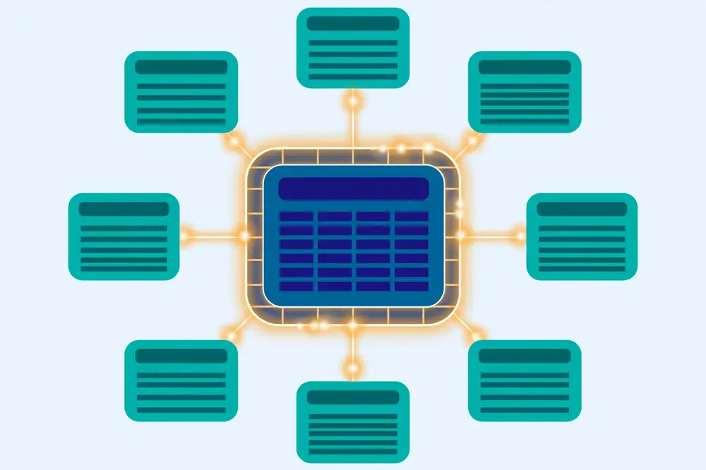
Figure: a star schema — one central fact table surrounded by dimension tables.

---

Chapter 4: Denormalization and Star Schemas

Chapter 3 taught you to normalize for correct writes. But analytical questions — "total sales by product category and month" — run against normalized models painfully: a simple question can require joining six tables, and every join is a chance for mistakes and slow performance. Denormalization is the deliberate, controlled reintroduction of redundancy to make reads fast and simple. The star schema is the standard pattern for doing it well.

Why analytical queries hate normalized models

Take the 3NF enrollment model from Chapter 3. To answer "average grade by department and semester," you join Enrollments → Students → Departments, plus a semester attribute somewhere. Now imagine 20 tables and a business user (or a tired researcher at midnight) writing that query. Problems:

• Join complexity: every question needs deep join knowledge; one wrong join double-counts.
• Performance: many joins over large tables are slow.
• Usability: non-technical users cannot self-serve; every question needs an expert.

Analytical workloads are read-heavy (thousands of queries, few writes), so we optimize for reads — the opposite trade-off from operational systems.

Denormalization: redundancy on purpose

Denormalization means storing some data redundantly to avoid joins. Example: in an analytical Sales table, storing CustomerCity directly on each sales row (copied from the customer record) instead of joining to Customers every time. The redundancy is managed: an ETL process refreshes it on a schedule, and everyone knows the analytical table is a derived copy, not the system of record.

Rules for safe denormalization: 1. Denormalize a copy of the data (the warehouse/mart), never the operational source. 2. Refresh it on a defined schedule so staleness is known and acceptable. 3. Document what is denormalized and why — future you will thank present you. 4. Never denormalize to fix a broken normalized model; fix the model first.

The star schema: facts in the center, dimensions around

A star schema has: - One fact table in the center (the measurements/events — Chapter 5 goes deep). - Dimension tables around it (the "by" in every question: by product, by customer, by date).

Text diagram of a retail star schema:

        DimProduct                  DimDate
   (ProductKey, Name,          (DateKey, Date, Month,
    Category, Brand)            Quarter, Year)
         \                        /
          \                      /
           \                    /
        ==== FactSales ====
        (DateKey FK, ProductKey FK,
         CustomerKey FK, StoreKey FK,
         Quantity, UnitPrice,
         SalesAmount)
           /                    \
          /                      \
         /                        \
   DimCustomer                DimStore
   (CustomerKey, Name,     (StoreKey, StoreName,
    City, Segment)          City, Region)

Every dimension connects directly to the fact table with a single join — one hop, never a chain. That is the entire secret of the star schema's simplicity and speed.

Star vs. snowflake

A snowflake schema normalizes the dimensions: DimProduct links to DimCategory, which links to DimDepartment — the star's points sprout sub-points, like a snowflake. Comparison:

Aspect	Star schema	Snowflake schema
Dimension tables	Denormalized, flat, wide	Normalized into sub-dimensions
Joins per query	Fewer (one hop to each dimension)	More (chains through sub-dimensions)
Query simplicity	High — business users cope	Lower — needs join expertise
Storage	More (redundancy in dimensions)	Less
Maintenance on hierarchy change	Update one wide table	Update small tables (cleaner)
Tool support (Power BI etc.)	Excellent — the preferred shape	Supported, but slower and more complex

Guideline: default to star. Snowflake only when a dimension hierarchy is genuinely volatile or enormous and the maintenance benefit outweighs the query cost. (A full comparison table also appears in the Learning Dashboard at the end of this book.)

Worked example: flattening a normalized model into a star

Normalized source tables: Orders(OrderID, CustomerID, OrderDate), Customers(CustomerID, Name, CityID), Cities(CityID, CityName, RegionID), Regions(RegionID, RegionName), OrderLines(OrderID, ProductID, Qty, Price), Products(ProductID, Name, CategoryID), Categories(CategoryID, CategoryName).

Star design: - DimCustomer(CustomerKey, CustomerName, City, Region) — Cities and Regions flattened in. - DimProduct(ProductKey, ProductName, Category) — Categories flattened in. - DimDate(DateKey, Date, Month, Quarter, Year, DayName) — built once, reused by every star in the warehouse. - FactSales(OrderLineKey, DateKey, CustomerKey, ProductKey, Quantity, UnitPrice, LineAmount) — one row per order line.

"Total sales by region and quarter" is now three one-hop joins and a SUM. A business user can build it by dragging fields in Power BI without writing a single join.

Conformed dimensions: the enterprise payoff

When every star schema in the warehouse shares the same DimDate and DimCustomer (same keys, same definitions), those are conformed dimensions. The payoff is huge: "sales by region" and "support tickets by region" use the same region definition, so the numbers agree. Building conformed dimensions is a one-time investment that ends the era of disagreeing reports from Chapter 1.

Galaxy schemas: when one star is not enough

Real warehouses have many fact tables sharing dimensions — sales facts, inventory facts, support-ticket facts all orbiting the same DimDate, DimProduct, DimCustomer. This multi-star arrangement is called a galaxy schema (or fact constellation). It is not a different technique — it is what you get when you build several star schemas with conformed dimensions. The design rule: dimensions are shared and identical; facts never join to each other directly (drill across instead, Chapter 7). If you find yourself building a second, slightly different DimCustomer for the support-ticket star, stop — conform the one you have.

Loading the star: ETL refresh patterns

A star schema is a derived copy, so you need a loading strategy:

• Full refresh: wipe and reload a table each cycle. Fine for small dimensions (a few thousand rows); simple and always consistent.
• Incremental load: load only new/changed rows, detected by a LastModified timestamp or source change-tracking. Essential for large fact tables — you cannot reload a billion-row fact nightly.
• Snapshot loads: for balances and statuses, capture the full state periodically into a periodic-snapshot fact (Chapter 5).
• Late-arriving data: facts sometimes arrive after their dimension rows (a sale recorded before the new customer's record syncs). Handle with an inferred-member pattern: create a placeholder dimension row, then update it when the real data arrives — or hold the fact in an error queue. Decide the policy; do not let late data silently vanish.

Refresh ordering matters: load dimensions before facts (facts need the keys), and expire Type 2 rows before inserting replacements (Chapter 6). A failed dimension load should block the fact load — loading facts against stale dimensions corrupts history.

Worked example: converting the snowflake to a star, concretely

Take the snowflaked chain FactSales → DimProduct → DimCategory → DimDepartment. The star conversion flattens the chain into one DimProduct built by a join at ETL time:

-- ETL: build the flattened dimension once per load
SELECT p.ProductID          AS ProductKey,   -- surrogate in practice
       p.ProductName,
       c.CategoryName       AS Category,
       d.DepartmentName     AS Department,
       p.Brand
FROM   Products p
JOIN   Categories c   ON c.CategoryID = p.CategoryID
JOIN   Departments d  ON d.DepartmentID = c.DepartmentID;

The result is stored as the physical DimProduct — the joins happen once per night in ETL, not once per query by every user. If a category is renamed, the ETL rebuilds the affected rows (and Type 2 versioning from Chapter 6 preserves history). This is the fundamental trade: pay the join cost once at load time instead of a thousand times at query time.

The date dimension: build it once, build it well

DimDate deserves special attention because every star uses it and time analysis is where models most visibly succeed or fail. A production-grade date dimension includes:

• Keys and dates: DateKey (integer YYYYMMDD — human-readable and sortable), Date (actual date type).
• Calendar hierarchy: Day, DayName, DayOfWeek, MonthNumber, MonthName, Quarter, Year, plus MonthYear ("Jan 2026") for axis labels.
• Fiscal hierarchy: FiscalMonth, FiscalQuarter, FiscalYear (if the organization uses one — never assume fiscal = calendar).
• Flags: IsWeekend, IsHoliday, IsWorkday — computed once, reused by every analysis ("sales on working days only").
• Relative markers: DaysAgo, IsCurrentMonth, IsYTD — optional conveniences for "last 30 days" logic.
• Coverage: every date from several years past to several years future, no gaps — gaps break time-intelligence functions silently.

Generate it with a script (SQL, Python, or Power Query — a few dozen lines), not by hand. Mark it as the date table in Power BI, hide the DateKey from report view, and set MonthName to sort by MonthNumber. This single table, done right, eliminates an entire category of Chapter 9 mistakes.

Aggregate fact tables: pre-computation for speed

When a transaction fact grows to hundreds of millions of rows, even star-schema queries slow down for high-level dashboards ("yearly sales by region" should not scan a billion rows). The answer is aggregate fact tables: pre-computed summaries at coarser grains, e.g., FactSalesMonthly(CityKey, ProductKey, MonthKey, TotalQty, TotalSales) — the same conformed dimensions, fewer rows by 100×. Modern engines (Power BI aggregations, materialized views) can route queries to the aggregate automatically when the question's grain allows, drilling through to detail on demand. Rules: aggregates must use identical dimension keys and definitions (or they are not the same numbers, just similar ones); every aggregate is documented as derived, with its grain stated; reconciliation checks compare aggregate totals to base-fact totals after each load. Aggregates are a performance technique, never a modeling shortcut — build the base fact first, aggregate second.

The ETL mapping document: from source to star

The bridge between the normalized source and the star is the mapping document — one row per target column:

Target table.column	Source	Transformation	Load rule
DimCustomer.City	crm.customers.city	Trim, title-case; map NULL → 'Unknown'	Type 2 on change
FactSales.SalesAmount	pos.order_lines.qty × price − discount	Convert to reporting currency (PKR) at daily rate	Reject if ≤ 0
DimDate (all)	Generated	Script gen_dates.py, 2020–2035	Full refresh yearly

Write the mapping before building the ETL — it forces every transformation decision into the open (currency conversion? null handling? rejection rules?) where stakeholders can review it. The mapping document plus the lineage diagram is the ETL specification; a developer should be able to build the pipeline from it without asking you a single question.

For your research: If your study produces repeated analytical cuts — survey waves, experiment conditions, sensor deployments — build yourself a small star: one fact table (responses, measurements) and flat dimensions (respondent attributes, question attributes, date, wave). Your analysis scripts become short, uniform aggregations (group by dimension, summarize fact), and adding wave 3 of a longitudinal study is just more fact rows, not a restructured spreadsheet. Reviewers can follow the logic because the shape is standard.

Key takeaways: - Normalize for correct writes; denormalize (in a separate analytical copy) for fast, simple reads. - A star schema = one central fact table + denormalized dimension tables, each one join away. - Prefer star over snowflake unless dimension maintenance genuinely demands normalization. - Conformed dimensions (shared across analyses) are how you get numbers that agree everywhere.

---

Chapter 5: Fact Tables vs Dimension Tables

The star schema's two table types do completely different jobs, and confusing them is one of the most common modeling errors. This chapter draws the line sharply, with rules for each and worked examples.

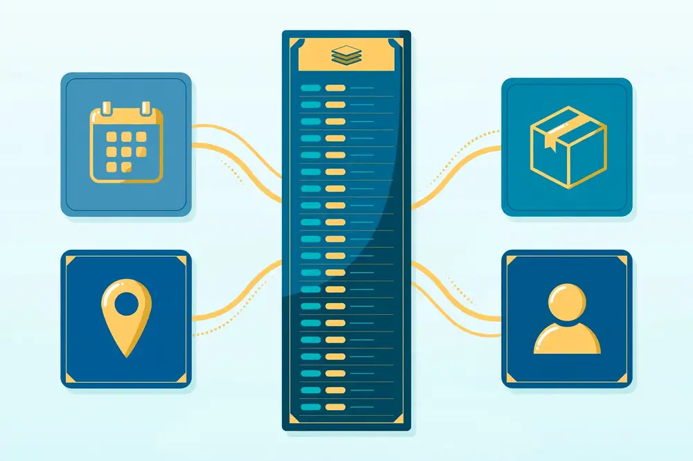
Figure: a fact table of measurable events surrounded by descriptive dimension tables.

The core distinction

• Fact tables record measurements of events: things that happened, quantified. Sales transactions, sensor readings, survey responses, website clicks, exam scores. Facts answer "how much / how many."
• Dimension tables describe the context of those events: who, what, where, when, why. Customers, products, stores, dates, respondents, questions. Dimensions answer "by what" — they are the slicing axes of every report.

Memory aid: facts are verbs (sold, measured, answered, clicked); dimensions are nouns (customer, product, date, question).

Anatomy of a fact table

A fact table has two kinds of columns and almost nothing else:

1. Foreign keys to dimensions (the grain-defining context): DateKey, ProductKey, CustomerKey, StoreKey.
2. Measures: numeric, additive-ish facts: Quantity, UnitPrice, SalesAmount, DiscountAmount.

What a fact table does not have: descriptive text attributes (product name, customer city — those live in dimensions), and usually no primary key in the analytical sense (the combination of dimension keys is the identity; some designers add a degenerate key like OrderLineNumber — see below).

Sample fact table — FactSales:

DateKey	ProductKey	CustomerKey	StoreKey	Quantity	UnitPrice	SalesAmount
20260105	501	9001	12	2	1500	3000
20260105	502	9002	12	1	95000	95000
20260106	501	9001	12	1	1500	1500

One row = one order line (that is the grain — Chapter 7). The foreign keys are the address; the measures are the payload.

The three kinds of facts

Not all measures behave the same under aggregation, and modeling them correctly matters:

1. Additive facts — can be summed across all dimensions. SalesAmount, Quantity. The well-behaved majority.
2. Semi-additive facts — can be summed across some dimensions but not others. Account balances sum across accounts but not across time (summing January's balance + February's balance is meaningless — you want the latest). Inventory levels are the classic example.
3. Non-additive facts — cannot be summed at all. Ratios, percentages, unit prices. UnitPrice summed across products is nonsense. Store these at the fact grain and compute ratios after aggregating the additive components (sum revenue ÷ sum quantity = correct average price; averaging the averages is wrong — a classic error).

Rule: store additive components in the fact table; compute ratios and percentages in measures/reports, never as stored summed values.

Anatomy of a dimension table

Dimensions are wide, descriptive, and relatively small:

• A surrogate primary key (CustomerKey) — meaningless integer, stable forever (Chapter 6 explains why this matters when attributes change).
• Descriptive attributes: names, categories, types, flags — the labels and groupings of reports.
• Hierarchies rolled into the same table (denormalized): Category, Subcategory, ProductName all in DimProduct; Year, Quarter, Month, Date all in DimDate.
• A row per member: one row per customer, per product, per date — including special rows like "Unknown" (key 0 or -1) so facts with missing dimension values still join cleanly instead of vanishing from reports.

Sample dimension — DimProduct:

ProductKey (PK)	ProductName	Category	Brand	UnitCost
501	Wireless Mouse	Electronics	LogiTech-style	900
502	Laptop 14"	Electronics	CompuBrand	78000

Factless fact tables and degenerate dimensions

Two special cases worth knowing:

• Factless fact tables record that an event happened but carry no measures — only foreign keys. Example: FactAttendance(StudentKey, DateKey, CourseKey) — one row per student per class session attended. The "measure" is the row count itself. Coverage/attendance/compliance scenarios use these constantly.
• Degenerate dimensions are dimension-like attributes with no table of their own — typically transaction numbers like OrderNumber or TicketNumber stored directly in the fact table. They have no attributes beyond the identifier, so a table would be pointless; but keep them in the fact because users filter and drill by them.

Worked example: modeling a research experiment

A psychology lab runs a reaction-time experiment: 60 participants, each completes 200 trials across 4 conditions, reaction time recorded per trial.

• Fact table FactTrials(ParticipantKey, DateKey, ConditionKey, TrialNumber, ReactionTimeMs, CorrectFlag) — one row per trial (grain = one trial). Measures: ReactionTimeMs (non-additive — average it, don't sum it), CorrectFlag (0/1, additive — sums to total correct).
• Dimensions: DimParticipant(ParticipantKey, Age, Gender, Group) (slowly changing — Chapter 6), DimCondition(ConditionKey, ConditionName, StimulusType), DimDate.

"Mean reaction time by condition for the experimental group" = filter DimParticipant.Group, group by DimCondition, average FactTrials.ReactionTimeMs. Clean, fast, and the shape scales to 60,000 trials without restructuring.

The three fact table types: transaction, snapshot, accumulating

Kimball's framework distinguishes three fact table types by what event the grain captures. Choosing correctly is one of the highest-leverage modeling decisions:

1. Transaction fact tables — one row per event at the moment it happens. FactSales (one row per order line), FactClicks (one row per click), FactResponses (one row per answer). The most common type; the grain is the event itself. Rows are inserted once and never updated. Analysis: counts, sums, trends over the event date.

2. Periodic snapshot fact tables — one row per thing per period, capturing state. FactInventorySnapshot(ProductKey, DateKey, QtyOnHand, QtyOnOrder) — one row per product per day, even with no transactions. This is how you answer "what was inventory on March 15?" — a transaction fact cannot answer state-at-a-point-in-time questions. Snapshots are dense (a row for every combination every period — large!) and carry semi-additive facts (Chapter 5: sum across products, not across days). Typical use: balances, headcounts, inventory, survey panel membership per wave.

3. Accumulating snapshot fact tables — one row per process, updated as the process moves through stages. FactOrderPipeline(OrderKey, OrderDateKey, ShipDateKey, DeliveryDateKey, OrderAmount, ShipLagDays, DeliveryLagDays) — one row per order, with a date key per milestone; the row is updated when the order ships, then again when delivered. Perfect for pipeline/lifecycle analysis: "average days from order to ship by month", "orders stuck in 'shipped' over 10 days". The grain is the process instance; multiple date roles (Chapter 8's role-playing dimensions) are the signature pattern.

How to choose:

Question to answer	Fact type
How many events happened?	Transaction
What was the state on date X?	Periodic snapshot
How long do processes take? Where do they stall?	Accumulating snapshot

Worked example — research grant applications: a funding body wants three analyses: (a) applications received per month → transaction fact FactApplications(ApplicationKey, DateKey, ApplicantKey, ProgramKey, RequestedAmount); (b) total pipeline value at each month-end → periodic snapshot FactPipelineSnapshot(ProgramKey, MonthKey, ApplicationsInReview, TotalRequested); (c) average days from submission to decision, and where applications stall → accumulating snapshot FactApplicationPipeline(ApplicationKey, SubmitDateKey, ReviewDateKey, DecisionDateKey, DaysToReview, DaysToDecision, Outcome). Three grains, three fact tables, one set of conformed dimensions — the galaxy pattern from Chapter 4.

Drilling down and rolling up: using the grain deliberately

Drill down moves from coarse to fine (year → quarter → month → day); roll up moves fine to coarse. Both are safe when the path follows the dimension hierarchy, because hierarchies are defined to aggregate cleanly. Drill through jumps from an aggregated number to the underlying fact rows ("show me the actual order lines behind this 2.4M") — invaluable for trust ("prove it") and for debugging. Drill across (Chapter 7) combines fact tables. A good model supports all four; a bad model supports none and forces users into raw table dumps.

Drill-across worked example: sales vs. targets, numerically

"Achievement % by city by month" drills across FactSales (order-line grain) and FactTargets (city-month grain) via conformed DimCity and DimDate. The engine's logic, step by step:

1. Aggregate FactSales to the common grain: SELECT CityKey, Month, SUM(SalesAmount) → (Karachi, 2026-06, 4,200,000).
2. Aggregate FactTargets (already at city-month): (Karachi, 2026-06, 5,000,000).
3. Join the two small result sets on CityKey + Month.
4. Compute the ratio on the joined result: 4,200,000 / 5,000,000 = 84%.

In DAX, Achievement % = DIVIDE([Total Sales], [Total Target]) does exactly this: each measure aggregates its own fact to the filter context's grain (city × month from the visual), then the division happens last. The critical insight: the join happens after aggregation, never before — that is what keeps different grains from corrupting each other. Any attempt to join the raw tables first (fan trap territory) multiplies rows and produces fiction. When a drill-across number looks wrong, check that both measures aggregate correctly independently before suspecting the combination.

Units, currencies, and other fact-table disciplines

Two details separate professional fact tables from amateur ones:

• One currency, one unit. A SalesAmount column mixing rupees, dollars, and euros is un-aggregatable. Standardize at ETL: store SalesAmount in a single reporting currency plus SalesAmountLocal and CurrencyCode if local values matter; document the exchange-rate source and date. The same for units: kilograms vs. grams, minutes vs. hours — pick one, convert at load, record the original in a companion column if needed.
• No null measures; no missing semantics. A NULL Quantity — does it mean zero, unknown, or not applicable? Decide per measure, encode it (0 vs. NULL vs. a QualityFlag), and document it. Aggregations treat NULL and 0 very differently (AVG ignores NULLs; SUM treats them as 0-ish absence), so ambiguity here silently corrupts statistics.

Add both checks to your ETL validation: "all amounts in reporting currency" and "no unexpected null measures." These are the boring rules that keep headline numbers trustworthy.

For your research: When you design your analysis dataset, explicitly label each table as fact or dimension and each numeric column as additive, semi-additive, or non-additive. This single exercise prevents the most embarrassing analysis errors: summed percentages, averaged totals, double-counted respondents. Put the labels in your data dictionary (Chapter 10) — reviewers who see "ReactionTimeMs: non-additive, report means only" will trust your statistics more.

Key takeaways: - Facts = measurable events (how much); dimensions = context (by what). Facts are verbs, dimensions are nouns. - Fact tables hold dimension foreign keys + numeric measures; dimension tables hold surrogate keys + descriptive attributes. - Classify measures: additive (sum freely), semi-additive (not across time), non-additive (compute ratios after aggregating). - Factless fact tables track event occurrence; degenerate dimensions (like order numbers) live in the fact table without their own table. - Label fact/dimension and additivity in your data dictionary — it prevents entire classes of analysis errors.

---

Chapter 6: Slowly Changing Dimensions — Types 1, 2, and 3

Real-world things change: customers move cities, products get rebranded, respondents change departments, sensors get recalibrated. A slowly changing dimension (SCD) is a dimension whose attributes change over time — "slowly" relative to the fact events. The modeling question is: when an attribute changes, do we overwrite history, keep history, or do a bit of both? The three classic answers are SCD Types 1, 2, and 3.

Why this matters: the history problem

Consider DimCustomer with customer 9001, Ali, living in Karachi. On March 1, he moves to Islamabad. In June you run "total 2026 sales by city." Should Ali's January purchases (made while he lived in Karachi) count under Karachi or Islamabad? There is no universally right answer — it depends on the business question — but your model must implement one answer deliberately, not produce a random one because nobody thought about it. That is what SCD types are for.

Type 1: overwrite — "only the present matters"

How it works: when the attribute changes, update the existing dimension row in place. History is rewritten.

Example — DimCustomer before and after Ali's move:

Before: | 9001 | Ali | Karachi | … | After: | 9001 | Ali | Islamabad | … |

All of Ali's facts — January's and June's — now roll up to Islamabad.

When to use: for corrections (a misspelled name, a wrongly entered city) and for attributes where history genuinely does not matter (a customer's current email for contact purposes).

Pros: simple; dimension stays small; always reflects current truth. Cons: history is destroyed — you can never again answer "as it was at the time." Dangerous if applied to attributes used in historical analysis.

Type 2: add a new row — "keep full history"

How it works: when a tracked attribute changes, insert a new dimension row with a new surrogate key; keep the old row. The fact table's foreign keys point to whichever row was current when the fact occurred. Rows carry effective dates and a current flag.

Example — DimCustomer as Type 2:

CustomerKey (PK)	CustomerID (natural)	Name	City	EffectiveFrom	EffectiveTo	IsCurrent
9001	C-100	Ali	Karachi	2024-01-01	2026-02-28	No
9007	C-100	Ali	Islamabad	2026-03-01	9999-12-31	Yes

Note the crucial mechanics: the surrogate key (CustomerKey) changes — that is what makes history work, because January's sales rows point to 9001 (Karachi) and June's point to 9007 (Islamabad). The natural key (CustomerID C-100) stays constant, so you can still find "all rows for Ali." January sales count under Karachi; June sales under Islamabad. Full history preserved.

When to use: whenever historical accuracy matters — customer segments, product categories, respondent demographics in longitudinal studies, anything a trend analysis might slice by.

Pros: complete history; "as was" and "as is" analyses both possible. Cons: dimension grows (one row per change); queries must usually filter IsCurrent = Yes for current-state reports; ETL is more complex.

Implementation notes: the ETL process compares incoming source records against the current dimension row; on a tracked-attribute change, it expires the old row (set EffectiveTo, IsCurrent = No) and inserts the new one. Untracked attributes (e.g., a phone number you do not analyze historically) can still be Type 1-overwritten even in a Type 2 dimension — hybrid handling per attribute is normal and should be documented.

Type 3: add a column — "keep the previous value"

How it works: keep two columns: current value and previous value. On change, shift current → previous, write the new current.

Example — DimCustomer as Type 3:

Before: | 9001 | Ali | CurrentCity: Karachi | PreviousCity: NULL | After: | 9001 | Ali | CurrentCity: Islamabad | PreviousCity: Karachi |

When to use: when you need exactly one step of history — "current vs. immediately previous" — e.g., a sales reorganization where you want this quarter vs. last quarter's territory assignment, no deeper.

Pros: simple; both values queryable in one row. Cons: only one generation of history; a second change destroys the original previous value; rarely the right choice — Type 2 is usually better and barely harder.

Choosing between the types

Question	Answer
Was it a data entry error?	Type 1 (overwrite the mistake)
Does any historical analysis slice by this attribute?	Type 2 (keep history)
Do we need only current vs. previous?	Type 3 (or Type 2 — simpler to stay consistent)
Is it just a contact detail nobody analyzes?	Type 1
Not sure?	Type 2 — history you keep can be ignored; history you destroy is gone forever

The golden rule: when in doubt, use Type 2. Storage is cheap; lost history is unrecoverable. You can always present a "current only" view over a Type 2 dimension, but you can never reconstruct history from a Type 1 overwrite.

Worked example: longitudinal survey study

A three-wave panel survey tracks respondents' employment status. Respondent R-014 is "Student" in Wave 1, "Employed" in Wave 2, "Employed" in Wave 3.

• Type 1 DimRespondent: R-014's row says "Employed." Wave 1 responses now appear to come from an employed person — wrong, and it corrupts any "responses by employment status at time of response" analysis.
• Type 2 DimRespondent: three rows for R-014 (or two: Student row effective Wave 1, Employed row effective Waves 2–3). Each FactResponses row points to the correct version. "How did employed respondents answer in Wave 1?" and "How do currently-employed respondents' answers trend across waves?" are both answerable — the second via the natural key.
• Document your choice in the methods section: "Respondent demographics were modeled as Type 2 slowly changing dimensions, preserving attribute values at time of response." Reviewers of longitudinal work notice and respect this.

Mini design exercise

DimProduct tracks Category and SupplierName. Marketing analyzes trends by category historically (needs history → Type 2 for Category). Procurement just needs the current supplier for reordering (Type 1 for SupplierName). One dimension, two treatments — document per attribute:

Attribute	SCD treatment	Reason
Category	Type 2	Historical trend analysis by category
SupplierName	Type 1	Only current value operationally needed
ProductName	Type 1	Corrections only

The Type 2 ETL process, step by step

Type 2 is conceptually simple but mechanically precise. Here is the load logic for DimCustomer, run each cycle:

1. Extract the current source record for natural key C-100: (Ali, Islamabad, Segment=Regular).
2. Look up the current dimension row (IsCurrent = Yes) for C-100: (Ali, Karachi, Segment=New).
3. Compare tracked attributes (City, Segment). City changed (Karachi → Islamabad) → a new version is needed. (Untracked attributes like phone are compared separately — changes there just overwrite, Type 1, even on a Type 2 row.)
4. Expire the old row: set EffectiveTo = yesterday, IsCurrent = No. Never delete it — facts still point to it.
5. Insert the new row: new surrogate key, EffectiveFrom = today, EffectiveTo = 9999-12-31, IsCurrent = Yes, natural key unchanged.
6. Route facts: new fact rows look up the current surrogate key at load time, so they automatically point to the right version.

Edge cases to handle: a change and a change-back (two new rows — correct, history is history); multiple changes in one load cycle (process in chronological order); a brand-new natural key (insert with no expiry step). Test the loader with a scripted scenario — "customer moves twice in one week" — before trusting it on real data.

Mini-dimensions and junk dimensions: taming high-cardinality attributes

Two refinements for dimensions that would otherwise explode under Type 2:

• Mini-dimension: when a large dimension (millions of customers) has a few frequently-changing attributes (age band, segment score), splitting those attributes into a small separate mini-dimension avoids versioning the giant table. DimCustomer keeps stable attributes; DimCustomerProfile(ProfileKey, AgeBand, Segment, ScoreBand) is Type 2 on its own; the fact table carries both keys. The profile dimension has only hundreds of rows (every combination of the few attributes).
• Junk dimension: leftover yes/no flags and codes that do not deserve their own tables (IsGiftWrap, ShipPriority, PaymentType, ReturnFlag) get bundled into one junk dimension — one row per observed combination. It keeps the fact table clean (one JunkKey instead of six flag columns) and gives the flags a browsable home.

Both are standard Kimball techniques: use them when a dimension is either too volatile or too scrappy for the clean Type 2 pattern.

Late-arriving dimensions and early-arriving facts

Sometimes a fact arrives before its dimension row (the sale syncs before the new-customer record). Options: (a) inferred member — create a placeholder dimension row ("Unknown, pending") with the natural key, then fill in attributes when they arrive (keeping the same surrogate key — this is one of the few legitimate in-place updates on a Type 2 dimension); (b) error queue — hold the fact until the dimension arrives, with alerting. Choose (a) when dimension delays are routine and minutes-long; (b) when they signal an upstream problem you want to see. Either way, decide and document — do not drop the fact silently.

Type 0 and Type 6: the ends of the spectrum

Two more types complete the picture:

• Type 0 — never change. The attribute is frozen at its first value (e.g., OriginalAcquisitionChannel, BirthDate). Even if the source sends an update, the loader ignores it. Use sparingly and deliberately — it is a business rule ("we always want the original value"), not laziness. Document it loudly, because it surprises people.
• Type 6 — the hybrid (1 + 2 + 3). Keeps the Type 2 history rows and adds a CurrentX column on every row holding the present value. This lets one query answer both "as was" (filter the historical row) and "as is" (read the Current column) without self-joining the dimension. It costs a little ETL complexity (every new version updates the Current column on all sibling rows) and is worth it for heavily-used dimensions where both perspectives are queried constantly.

Choosing across all types: Type 0 for frozen origin facts; Type 1 for corrections and current-only attributes; Type 2 as the default for anything analyzed historically; Type 3 for the rare current-vs-previous-only need; Type 6 when "as is" and "as was" are both hot query paths. Most real dimensions use a mix per attribute — the per-attribute SCD table from this chapter's mini exercise is the document that records the mix.

Testing SCD logic: scenarios that catch bugs

SCD loaders fail in predictable ways — test for them explicitly:

1. The double move: customer changes city twice between loads. Expected: two new versions, ordered by effective date, no gaps or overlaps in coverage.
2. The change-back: city changes Karachi → Islamabad → Karachi. Expected: three versions; history shows the truth, not a net-zero.
3. The midnight boundary: change effective exactly at a fact's timestamp. Expected: deterministic rule (e.g., facts on the effective date use the new version) applied consistently.
4. The untracked change: phone number updates. Expected: overwrite in place, no new version, history of tracked attributes untouched.
5. The late correction: source corrects last month's city. Expected: per your policy — either restate history (new versions with corrected dates) or leave history and fix forward. Both are defensible; silent in-place edits of expired rows are not.

Automate these as a test fixture with a tiny synthetic dimension. SCD bugs are silent — totals still compute, reports still render — so only scenario tests catch them.

For your research: Any study running longer than a few months has slowly changing dimensions: respondents change institutions, sensors get recalibrated, experimental protocols get revised. Decide before data collection which attributes need history. The cheapest implementation is a Type 2 pattern in a spreadsheet or SQLite table: add EffectiveFrom, EffectiveTo, IsCurrent columns and never update a row in place — always expire and insert. Your future self, writing the longitudinal analysis chapter, will be profoundly grateful.

Key takeaways: - SCDs handle dimension attributes that change over time; the question is always what happens to history. - Type 1 overwrites (history lost) — for corrections and current-only attributes. - Type 2 adds a new row with a new surrogate key (full history) — the default choice for anything analyzed historically. - Type 3 keeps current + previous columns — only for single-step history needs. - When in doubt, Type 2: kept history can be ignored, destroyed history cannot be recovered. - Document the SCD type per attribute in your data dictionary.

---

Chapter 7: Hierarchies, Granularity, and Grain Statements

If Chapter 2 gave you tables and keys, this chapter gives you the discipline that holds a model together: knowing exactly what one row means (grain), how detailed your data is (granularity), and how attributes roll up into bigger groups (hierarchies). Grain mistakes are the number-one cause of wrong numbers in analytical models — this chapter makes sure you never make one.

Grain: what does one row mean?

The grain of a table is the precise definition of what a single row represents. It is the most important sentence in any data model, and it should be written down explicitly as a grain statement. Examples:

• FactSales: "One row per product per order line."
• FactAttendance: "One row per student per course per class session."
• FactSensorReadings: "One row per sensor per 5-minute interval."
• DimCustomer (Type 2): "One row per customer per version of tracked attributes."

The grain test: pick any row in the table and check it against the statement. If you find a row that represents something else, the grain is broken (or the statement is wrong). A table with mixed grain — some rows daily, some monthly — is a time bomb: every aggregation over it is wrong in ways that are hard to detect.

Granularity: the level of detail

Granularity is how fine or coarse the data is: transaction-level (finest), daily summaries, monthly summaries (coarsest). Higher granularity (finer detail) is more flexible — you can always roll daily data up to months, but you can never drill monthly data down to days. Rule: capture data at the finest grain you can afford; aggregate later. Storage is cheap; lost detail is permanent.

This has a direct research parallel: record raw trial-level data even if you plan to analyze participant means. The participant means can always be computed; the trial-level patterns (learning curves, outlier trials) cannot be recovered from means.

Hierarchies: rolling up

A hierarchy is a chain of attributes from fine to coarse within a dimension: Day → Month → Quarter → Year in DimDate; Product → Subcategory → Category → Department in DimProduct; Village → District → Province in a geography dimension. Hierarchies power drill-down in reports (year → quarter → month) and must be:

• Complete: every product has a category; no NULLs breaking the chain (use "Unknown" members instead).
• Consistent: the rollup path is the same for every row — a month belongs to exactly one quarter.
• Documented: note where hierarchies are ragged (real-world irregularities). Example: a university hierarchy Faculty → Department works until an interdisciplinary center reports to two faculties. Document the exception and the rule you applied.

Balanced vs. unbalanced hierarchies: a balanced hierarchy has the same depth everywhere (every date has day/month/quarter/year). An unbalanced (ragged) hierarchy varies: an org chart where some branches are 3 levels deep and others 6. Tools handle these differently — in Power BI, ragged hierarchies need careful modeling (parent-child hierarchies or flattened paths). Know which kind you have.

The grain matrix: a design tool

Before building, list your business processes and candidate grains in a grain matrix:

Business process	Candidate grain	Grain statement
Retail sales	Order line	One row per product per order
Website visits	Page view	One row per page view per session
Support tickets	Ticket	One row per ticket
Ticket status changes	Status change	One row per ticket per status change

Notice tickets appear twice: the ticket grain (current state, one row per ticket) and the status change grain (history, one row per change) are two different fact tables at two different grains. One fact table = one grain. When tempted to mix, create a second fact table instead.

Drilling across fact tables: the conformed-dimension contract

"Total sales vs. total support tickets by region and month" combines two fact tables at different grains (order line vs. ticket). This works — it is called drilling across — only if both facts share conformed dimensions (the same DimDate, the same DimRegion with the same keys). The query aggregates each fact to the common grain (region × month) and then joins the results. Without conformed dimensions, drilling across produces mismatched, meaningless comparisons. This is why Chapter 4's conformed dimensions matter so much.

The classic grain errors (and how to spot them)

Error 1: Fan-out (double counting). Joining a fact table to a dimension at the wrong grain multiplies rows. Example: FactSales (one row per order line) joined to a DimPromotions bridge where one order line matched two promotions → the sales amount appears twice in the total. Symptom: totals inflate after adding a table. Fix: check the join grain; use distinct-count-safe patterns or allocate measures properly.

Error 2: Mixed grain in one table. Daily rows and monthly summary rows coexisting in FactSales. Symptom: month totals that do not equal the sum of days. Fix: separate tables per grain, or a grain-identifying column with strict filtering — separate tables are cleaner.

Error 3: Chasm traps and fan traps. A fan trap: joining two fact-like tables through a shared dimension incorrectly — e.g., Customers → Orders → OrderLines is fine (a chain), but joining Orders directly to Shipments through Customer when the real path is through Order creates a fan that multiplies. A chasm trap: two fact tables sharing a dimension but with no direct relationship — "sales by customer" and "tickets by customer" cannot be joined row-to-row; they must each aggregate to customer first (drilling across). Fix: model the real relationships; aggregate before combining.

Worked check: given FactSales at order-line grain and DimDate at day grain, "sales by month" aggregates 30 daily rows into one month — safe, because month is coarser than the fact grain. Going the other direction — allocating a monthly target down to days — requires an explicit allocation rule, not a join. Roll up freely; allocate deliberately.

Parent-child and ragged hierarchies

Not all hierarchies are neat. A parent-child hierarchy stores each member with a pointer to its parent (the self-referencing pattern from Chapter 2: Employee → Manager). An org chart or a chart of accounts works this way — depth varies by branch, members can be added at any level. The modeling challenge: analytical tools want fixed levels (Level1, Level2, Level3 columns) but parent-child data has variable depth. Solutions: (a) flatten to a fixed number of levels in ETL (works if depth is bounded, e.g., ≤ 6); (b) use the tool's parent-child support (Power BI's PATH() DAX functions); (c) store both — the parent pointer for maintenance, flattened levels for querying. Document the maximum depth and what happens if it is exceeded.

A ragged hierarchy skips levels: a geography City → Province → Country where city-states have no province (NULL level). Options: fill with a placeholder ("N/A — city-state"), or use a parent-child representation. Never leave the level NULL without a policy — NULLs break drill paths silently.

Multiple hierarchies, one dimension

DimDate typically carries several hierarchies at once: calendar (Day → Month → Quarter → Year), fiscal (Day → Fiscal Month → Fiscal Quarter → Fiscal Year), and weekly (Day → Week → Year). They coexist as separate column sets in the same table — no new tables needed. The same applies to DimProduct (category hierarchy vs. brand hierarchy) and geography (administrative vs. sales-territory hierarchy). Rule: one dimension table, as many hierarchy column-sets as needed — the table is the conformed entity; the hierarchies are just different ways to roll it up. Name them unambiguously (FiscalQuarter vs. CalendarQuarter) so users never mix them.

Worked example: grain matrix for a hospital study

A research team models hospital operations data:

Business process	Fact table	Grain statement
Admissions	FactAdmissions	One row per patient per admission
Lab tests	FactLabTests	One row per admission per test per order time
Daily census	FactCensusSnapshot	One row per ward per day (periodic snapshot)
Patient journey	FactJourney	One row per admission, updated at discharge (accumulating snapshot)

Four processes, four grains, four fact tables — sharing DimPatient (Type 2), DimDate, DimWard, DimTest. "Average length of stay by ward by month" drills across FactJourney (accumulating) and DimDate; "tests per admission" drills across FactLabTests and FactAdmissions at the admission grain. The matrix is the design document the whole team signs off on before anyone builds.

The bus matrix: planning conformed dimensions enterprise-wide

When several teams build stars, the bus matrix keeps them conformed: rows are business processes (fact tables), columns are dimensions, and a check mark means "this process uses this dimension."

	DimDate	DimCustomer	DimProduct	DimStore	DimPromotion
FactSales	✓	✓	✓	✓	✓
FactInventory	✓		✓	✓
FactSupportTickets	✓	✓	✓

The matrix is built in a workshop before modeling begins, and it has a political function as much as a technical one: every team agrees on shared dimension definitions up front, which is what makes "sales by region" and "tickets by region" comparable later. A new fact table (a new row) reuses existing columns rather than inventing parallel dimensions. For a research group running multiple studies, the equivalent is a shared codebook: the same respondent, institution, and wave dimensions across projects, so findings compound instead of fragmenting.

Grain discipline in SQL: GROUP BY as a contract

In SQL, grain errors surface in GROUP BY. The discipline: the GROUP BY clause must match the grain you claim. If FactSales is at order-line grain and you want monthly category totals:

SELECT d.MonthName, p.Category, SUM(f.SalesAmount) AS TotalSales
FROM FactSales f
JOIN DimDate d     ON d.DateKey = f.DateKey
JOIN DimProduct p  ON p.ProductKey = f.ProductKey
GROUP BY d.MonthName, p.Category;

The grouped columns (Month, Category) are coarser than the fact grain — safe roll-up. Red flags in review: grouping by a fact's degenerate column (OrderNumber) while summing (double-counts across lines); joining a bridge table before aggregating (fan-out); SELECT DISTINCT used to "fix" inflated totals (masks the grain error instead of fixing it). A useful audit query: compare COUNT(*) to COUNT(DISTINCT <grain columns>) on the fact table — any difference means duplicate grains, and every downstream total is suspect until resolved.

For your research: Write a grain statement for every dataset you analyze, and put it in your methods section or data dictionary. "The analysis dataset contains one row per participant per trial (N = 12,000 rows; 60 participants × 200 trials)" tells a reviewer exactly what your N means at every level — and prevents the classic error of treating 12,000 trials as 12,000 independent participants in a statistical test. Grain discipline is statistical discipline.

Key takeaways: - Grain = what one row means. Write it as an explicit grain statement for every table. - Capture the finest grain affordable; you can roll up but never drill down beyond what was captured. - Hierarchies must be complete, consistent, and documented — note ragged exceptions. - One fact table = one grain; combine fact tables only via conformed dimensions (drilling across). - Fan-out double-counting, mixed grains, and fan/chasm traps are the classic grain errors — aggregate at a common grain before combining.

---

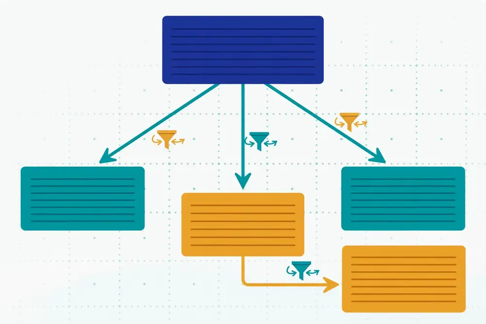
Figure: table relationships with cardinality and filter direction — the heart of a Power BI model.

---

Chapter 8: Building Models in Power BI — Relationships, Cardinality, Cross-Filter Direction

Power BI is where many researchers first meet data modeling in practice: you load tables, and Power BI asks you to define relationships between them. Get this right and DAX measures become simple; get it wrong and every visual shows wrong numbers with no error message. This chapter is the complete practical guide.

The model view: your blueprint in Power BI

Power BI Desktop's Model view shows your tables as boxes and relationships as lines — it is the visual form of everything in Chapters 2–7. A healthy model looks like a star: fact tables in the center, dimensions around, lines radiating outward. If your model view looks like spaghetti — tables chained in long lines, lines crossing everywhere — that is the tool telling you the model needs work.

Relationships: the four settings that matter

Every relationship in Power BI has four properties you must set deliberately:

1. The columns. Pick the key columns on each side — almost always the surrogate keys (DimCustomer[CustomerKey] ↔ FactSales[CustomerKey]). Both columns should contain matching values; data type mismatches (text vs. number) silently break joins — Power BI may auto-create a relationship on the wrong columns if names match, so verify every auto-detected relationship.

2. Cardinality. Three options: - One-to-many (1:*): DimCustomer (one) → FactSales (many). The standard, correct choice for dimension-to-fact. The "one" side should have unique values — Power BI will warn you if it does not. - One-to-one (1:1): both sides unique. Rare; used for the split-table scenarios in Chapter 2. - Many-to-many (:): both sides have duplicates. Sometimes legitimate (bridge patterns), but often a sign the model needs a bridge table or a grain fix. Power BI handles : with an internal bridge, but treat it as a yellow flag and verify totals carefully.

3. Cross-filter direction. This controls which way filters flow: - Single direction (dimension → fact): the default and usually correct. Selecting "Electronics" in a DimProduct slicer filters FactSales to electronics rows. Filters flow downhill from dimensions to facts. - Both directions (bi-directional): filters also flow from fact to dimension and across to other dimensions. This enables patterns like "show me customers who bought electronics" filtering a customer list — but it is dangerous as a default.

4. "Make this relationship active." Only one active relationship can exist between a given pair of tables along the same path. Multiple date roles (OrderDate, ShipDate) need inactive relationships activated selectively with USERELATIONSHIP() in DAX — or better, role-playing dimensions (see below).

Why "bi-directional everywhere" is the classic Power BI mistake

New modelers set every relationship to bi-directional because it makes more visuals "work" — filters seem to flow everywhere. The problems:

• Ambiguous filter paths: with bi-directional filters, a filter can reach a table via two different routes, and Power BI may error ("ambiguous relationship") or pick a path you did not intend.
• Performance: bi-directional relationships expand the filter context dramatically; large models slow down.
• Wrong results: filters flowing uphill from facts to dimensions can produce subtly wrong distinct counts and totals.

Rule: single direction everywhere; add bi-directional only for a specific, tested need (the classic legitimate case: a many-to-many bridge where filters must cross the bridge, or a specific "filter the dimension by fact" visual — implement it, test the totals, document why).

Role-playing dimensions: one date table, many roles

FactSales has OrderDateKey and ShipDateKey — two roles for dates. Do not import DimDate twice (that creates two competing date tables and confused users). Instead: import one DimDate, create one active relationship (to OrderDateKey) and one inactive relationship (to ShipDateKey). DAX measures for shipped amounts use CALCULATE([Total Sales], USERELATIONSHIP(DimDate[DateKey], FactSales[ShipDateKey])). Alternatively, create lightweight role-playing views (a SQL view or Power Query reference of DimDate named Ship Date) with single active relationships — simpler for business users, slightly more tables. Either is correct; duplicating the physical date logic is not.

Handling the standard tricky patterns

Many-to-many done right: Students ↔ Courses via Enrollments. In Power BI: DimStudent 1: Enrollments :1 DimCourse, with the bridge's filter direction set so slicers on either dimension filter the bridge. Measures count bridge rows or aggregate facts through it. Test with a matrix: students × courses should show the right intersections, and totals must equal the unfiltered total.

Inactive relationships and USERELATIONSHIP: covered above with dates. The pattern generalizes: any time two tables need two different join paths, one is active, the rest inactive and invoked per-measure.

Dealing with the date table: every Power BI model needs a proper date table — continuous dates with no gaps, marked as a date table, with Year/Quarter/Month/Day columns and useful flags (IsWeekend, IsHoliday). Do not use the fact's raw date column for time intelligence; DAX time functions (DATESYTD, SAMEPERIODLASTYEAR) require a proper date table. Build it once in Power Query or DAX (CALENDAR/CALENDARAUTO) and conform it across models.

Row-level security (RLS): filters applied per user role (a regional manager sees only their region). RLS is defined on dimension tables and flows downhill through single-direction relationships — another reason single direction is the default. Test every role with "View as" before publishing.

A step-by-step: modeling the retail star in Power BI

1. Load DimDate, DimProduct, DimCustomer, DimStore, FactSales via Power Query. Check data types: keys as whole numbers (or text consistently), dates as dates.
2. Hide key columns from report view (right-click → Hide) — users should see ProductName, not ProductKey. Keep keys visible only in Model view.
3. Create relationships: DimDate[DateKey] → FactSales[DateKey] (1:*, single); same for Product, Customer, Store. Verify the "one" side shows unique values.
4. Set sort order for month names: sort MonthName by MonthNumber, else April sorts before January alphabetically.
5. Write base measures: Total Sales = SUM(FactSales[SalesAmount]), Total Qty = SUM(FactSales[Quantity]). Never drag raw numeric columns into visuals when a measure will do — measures carry business logic in one place.
6. Test the grain: a card visual with Total Sales (no filters) must equal the source system's total. A matrix of Category × Month must sum to the same total. If not, stop — the model has a grain or relationship problem, not a DAX problem.
7. Document: rename tables/measures in business language, add descriptions (the field wells show them), organize measures in display folders.

Performance basics that are really modeling

• Star schema beats snowflake in Power BI's engine (VertiPaq) — fewer, wider tables compress and scan better.
• Reduce cardinality: the fewer unique values in a column, the better compression. Split datetime into date + time-of-day if you do not filter by second.
• Avoid bi-directional unless justified (see above).
• Hide unused columns, especially high-cardinality text columns nobody filters by.
• Aggregate tables for very large facts: a monthly summary table that Power BI uses automatically when the query grain allows.

Essential DAX measure patterns for a modeled star

With a clean star, most measures follow a few patterns. Learn these five and you cover 90% of reporting:

-- 1. Base additive measure
Total Sales = SUM ( FactSales[SalesAmount] )

-- 2. Ratio computed AFTER aggregation (never stored)
Avg Unit Price = DIVIDE ( [Total Sales], [Total Qty] )

-- 3. Distinct counts (note: slower on huge tables)
Active Customers = DISTINCTCOUNT ( FactSales[CustomerKey] )

-- 4. Time intelligence (needs the proper date table)
Sales YTD = TOTALYTD ( [Total Sales], DimDate[Date] )
Sales Last Year = CALCULATE ( [Total Sales], SAMEPERIODLASTYEAR ( DimDate[Date] ) )

-- 5. Inactive relationship (role-playing date)
Shipped Sales =
CALCULATE ( [Total Sales],
    USERELATIONSHIP ( DimDate[DateKey], FactSales[ShipDateKey] ) )

Notice how every pattern assumes the model from this book: single-direction 1: relationships, a conformed date table, additive base measures. DAX is easy when the model is right and miserable when it is wrong* — most "DAX problems" are modeling problems wearing a disguise.

Troubleshooting: the modeler's diagnostic guide

Symptom	Likely cause	Fix
Measure returns blank	Relationship on wrong columns; data-type mismatch; inactive relationship not activated	Check Model view lines; verify key data types match
Total changes when an unrelated slicer is added	Bi-directional filter path; ambiguous relationships	Set single direction; remove ambiguous paths
"Ambiguous relationship" error	Two filter paths between tables	Keep one active path; others inactive
Month sorts alphabetically	MonthName sorted by itself	Sort MonthName by MonthNumber column
YTD / SAMEPERIODLASTYEAR blank	No proper date table; gaps in dates	Build continuous DimDate; mark as date table
Visual is very slow	Bi-directional everywhere; high-cardinality columns; snowflake chains	Single direction; star schema; hide unused columns
Totals do not match source	Fan-out join; mixed grain; dropped NULL keys	Reconcile grain; add Unknown members; check joins

Work through this table top to bottom before rewriting any DAX — the fix is in the model nine times out of ten.

DirectQuery and composite models: a word of caution

Power BI's default Import mode loads data into its fast in-memory engine — ideal for star schemas up to millions of rows. DirectQuery leaves data in the source database and translates every click into SQL — necessary for real-time or huge data, but every visual becomes a live query, so model shape matters more, not less (a snowflake in DirectQuery is painfully slow). Composite models mix both. For research datasets, Import mode is almost always right: your data fits in memory, refreshes are simple, and DAX works fully. Choose DirectQuery only when data freshness or size genuinely demands it.

Organizing the model for humans: folders, descriptions, hierarchies

A technically correct model that users cannot navigate still fails. In Power BI's Model view:

• Display folders: group measures (Sales, Targets, Time Intelligence) so the field list stays navigable at 50+ measures. One flat list of 80 measures is unusable.
• Descriptions: every measure and key column gets a one-line description ("Total sales incl. tax, additive across all dimensions"). It appears as a tooltip — the cheapest documentation there is.
• Hierarchies: define drill hierarchies explicitly (Year → Quarter → Month → Day; Category → Subcategory → Product) so users drill with one click instead of adding columns manually.
• Hide ruthlessly: keys, intermediate columns, and ETL artifacts hidden from report view. The field list should show business concepts, not plumbing.
• Calculation groups (advanced): for repetitive time logic (YTD, last year, % change) defined once and applied to any measure — the DRY principle for DAX. Learn these after the fundamentals are solid.

Treat the field list as a user interface: if a new user cannot find "total sales by month" in 30 seconds, the model's presentation needs work regardless of its technical quality.

Publishing and refresh: the model goes live

A model is not done when it works on your laptop. Publishing checklist:

• Dataset settings: scheduled refresh aligned with source availability (nightly ETL → morning refresh); refresh failure alerts to the owner, not to a void.
• Gateways: on-premises sources need a data gateway; test refresh from the service, not just Desktop — credentials and paths differ.
• RLS roles: define roles on dimensions, test with "View as" for each role, and document who belongs where. RLS on a fact table instead of its dimensions is a common error — filters must flow downhill.
• Endorsement and discovery: certify the dataset as the sanctioned source ("use this, not the spreadsheet") — organizational trust is a feature you ship.
• Version note: keep a one-line dataset description with the model version and last refresh date, visible to consumers. "v3.2, refreshed 2026-10-08 06:00" prevents a week of confusion when numbers move.

For your research: Power BI (free Desktop version) is an excellent tool for exploratory analysis of research data and for building the charts in your thesis defense. Model your survey data as a star (Chapter 4's research example), set single-direction relationships, write explicit measures (Response Rate = DIVIDE(COUNT(FactResponses[ResponseID]), [Eligible Count])), and test totals against your raw data before trusting any visual. A screenshot of a clean star-schema Model view in your thesis appendix is a strong, concrete signal of data management rigor.

Key takeaways: - A healthy Power BI model looks like a star: facts centered, dimensions around, single-direction relationships. - Set four things deliberately per relationship: columns, cardinality (1:* dimension→fact), cross-filter direction (single by default), active/inactive. - Bi-directional everywhere causes ambiguity, slowness, and wrong totals — justify each exception. - One date table with role-playing (inactive relationships + USERELATIONSHIP) beats duplicated date tables. - Test the model before the DAX: totals must match the source, and matrices must foot to the grand total.

---

Chapter 9: Common Modeling Mistakes and How to Avoid Them

This chapter is a field guide to the errors that experienced modelers see again and again — each with symptoms, diagnosis, and fix. Use it as a checklist before you call any model "done."

Mistake 1: No grain statement (the root of all evil)

Symptom: two analysts compute "total sales" and get different numbers; nobody can explain why. Cause: the fact table's grain was never defined, so rows mean different things in different loads. Fix: write the grain statement; add a data-quality check that fails the load if a row violates it.

Mistake 2: Using names as keys

Symptom: "Ali" the customer merged with "Ali" the supplier; a renamed product splits its history in two. Cause: natural text used as a join key. Fix: surrogate integer keys everywhere in the analytical model; keep natural keys as attributes for searching.

Mistake 3: The spreadsheet-shaped model (repeating groups)

Symptom: columns named Q1…Q40, Jan…Dec, Phone1, Phone2; adding a question/month/phone requires schema surgery. Cause: 1NF violation carried into the model. Fix: reshape to rows (Chapter 3). In Power BI, unpivot in Power Query.

Mistake 4: Bi-directional relationships everywhere

Symptom: ambiguous-relationship errors, slow refresh, totals that change when you add an unrelated slicer. Cause: covered in Chapter 8 — filters flowing uphill through every relationship. Fix: single direction by default; bi-directional only where specifically needed and tested.

Mistake 5: Joining at the wrong grain (fan-out)

Symptom: revenue doubles when you add the promotions table to a visual. Detailed example: FactSales has 1,000 rows totaling 500,000. BridgeOrderPromotions maps some order lines to two promotions each. Joining at order-line grain duplicates those rows → total becomes 620,000. The report looks fine; the number is fiction. Fix: verify every join's grain; when a many-to-many genuinely exists, decide the allocation rule explicitly (split evenly? attribute to first?) and document it — never let the join decide silently.

Mistake 6: Two date tables (or none)

Symptom: time-intelligence measures return blanks; "month" sorts alphabetically; fiscal vs. calendar confusion. Fix: one conformed DimDate per model, marked as date table, with all needed attributes and roles handled via inactive relationships.

Mistake 7: Storing computed ratios in fact tables

Symptom: "average discount %" summed across regions gives 340%; nobody notices for months. Cause: non-additive facts (Chapter 5) stored and then summed. Fix: store additive components; compute ratios in measures after aggregation.

Mistake 8: NULL dimension keys silently dropping rows

Symptom: total in the dashboard is slightly less than the source total; the gap is the "unknown" rows that failed to join. Fix: "Unknown" member rows in every dimension (key −1/0) and ETL that maps unmatched keys to them; add a reconciliation check (fact total vs. source total) to every load.

Mistake 9: Snowflaking by habit

Symptom: simple questions need four joins; business users give up and go back to spreadsheets. Fix: default to star; snowflake only with a documented maintenance reason (Chapter 4).

Mistake 10: No documentation (the model only exists in one person's head)

Symptom: the modeler leaves; the model becomes untouchable; every change is feared. Fix: Chapter 10 — document as you build, not after.

Mistake 11: Mixing facts and dimensions in one table

Symptom: a "Sales" table with customer names, product categories, and amounts; every change to a product name requires updating a million rows. Fix: separate facts from dimensions (Chapter 5).

Mistake 12: Ignoring slowly changing dimensions until it is too late

Symptom: "sales by customer segment" history rewrites itself every time segments are redefined; trend analyses are meaningless. Fix: decide SCD types during design (Chapter 6), not after the first reorganization.

The pre-flight checklist

Before publishing any model, run through this:

• [ ] Grain statement written for every fact table
• [ ] Surrogate keys on all dimensions; no text keys in joins
• [ ] No repeating-group columns (Q1…Q40 patterns)
• [ ] Relationships: 1:* dimension→fact, single filter direction (exceptions documented)
• [ ] One conformed date table; roles via inactive relationships
• [ ] Measures classified additive/semi/non-additive; ratios computed, not stored
• [ ] "Unknown" members in dimensions; reconciliation totals match source
• [ ] Star schema (or documented reason for snowflake)
• [ ] SCD types decided per attribute
• [ ] Data dictionary started (Chapter 10)

Case study: rescuing the "Sales_FINAL_v2" model

A realistic rescue, step by step. You inherit a Power BI file from a departed colleague. Symptoms: the revenue total disagrees with finance by 18%; adding the Region slicer changes the grand total; some months show no data; nobody dares touch it.

Diagnosis (one hour in Model view): 1. No date table — visuals use FactSales[OrderDate], a raw datetime with gaps; time intelligence is broken (Mistake 6). 2. DimCustomer uses customer name as the key; two "Ali Traders" merged into one (Mistake 2). 3. Every relationship is bi-directional; Region slicer filters uphill through facts into other dimensions, shifting totals (Mistake 4). 4. FactSales contains a DiscountPct column that someone summed in a visual → 340% "total discount" (Mistake 7). 5. Promotion analysis joins at order grain to a line-grain fact → fan-out inflating revenue 18% (Mistake 5). 6. No documentation; the ETL is a chain of undocumented Power Query steps (Mistake 10).

The rescue plan (in order — sequence matters): 1. Freeze the current file as Sales_FINAL_v2_ARCHIVE — never operate without a rollback. 2. Build a proper DimDate; re-point all time analysis at it. 3. Introduce surrogate CustomerKey; remap facts; keep name as attribute. 4. Set all relationships to single direction; re-test each visual's totals. 5. Fix the promotion join: move to line grain with a documented allocation rule; reconcile to finance's 800K-equivalent figure until it matches to the rupee. 6. Replace the summed DiscountPct with a proper Avg Discount % = DIVIDE(SUM(DiscountAmount), SUM(GrossAmount)) measure. 7. Write the data dictionary and grain statements as you go — the rescue produces the documentation the original never had. 8. Run the pre-flight checklist; get finance to sign off on the reconciled total.

Lesson: every item in the rescue maps to one chapter of this book. Modeling knowledge is debugging knowledge — the same principles that build a good model diagnose a broken one. When you inherit a mess, resist the urge to rebuild from zero immediately: diagnose first (the business logic buried in the mess is valuable), then rebuild deliberately with the checklist.

Mistake 13: Modeling without stakeholders (the elegant irrelevance)

Symptom: a technically beautiful model that answers questions nobody asks; users keep their spreadsheets. Cause: the modeler designed from the source system's structure instead of from users' questions — the model mirrors the database, not the business. Fix: start every engagement with the question list (Chapter 1's workflow, step 1). Validate the conceptual sketch with actual users before building. A model is a communication tool first and a technical artifact second.

Mistake 14: Over-engineering (the framework astronaut)

Symptom: a seven-table snowflake where a three-table star would do; generic "flexible" structures (entity-attribute-value tables) that make every query a puzzle; SCD Type 6 on attributes nobody will ever analyze historically. Cause: designing for imagined future requirements instead of real ones. Fix: model for the questions you have, with sensible extension points (surrogate keys, a date dimension with room to grow). YAGNI — "you aren't gonna need it" — applies to data models too. Simple models get used; clever models get abandoned.

Mistake 15: No data-quality checks at load (garbage in, gospel out)

Symptom: the dashboard confidently shows wrong numbers for weeks before anyone notices; every fix is reactive. Cause: the ETL loads whatever the source sends — duplicates, negative quantities, future dates, orphaned keys — with no validation. Fix: a validation layer on every load, with three outcomes: reject (bad rows quarantined, load fails loudly — e.g., duplicate primary keys), warn (load continues, owner notified — e.g., 2% null emails, within tolerance), accept. Standard checks: row counts within expected bounds, key uniqueness, referential integrity (no orphaned foreign keys), value ranges (Qty > 0, dates not in the future), and the reconciliation total vs. source. Log every check result with the load — the log is your alibi when numbers are questioned.

The reconciliation habit: trust but verify, every time

The single highest-value habit in this book: after every load, reconcile. Fact row counts vs. source counts. Sum of SalesAmount vs. the source system's total. Dimension counts vs. yesterday (a 10× jump means something broke). Keep a tiny reconciliation table — LoadDate, TableName, RowCount, TotalAmount, Status — and review it like a pilot's checklist. Models with reconciliation catch corruption in hours; models without it catch corruption when a stakeholder does, which is the worst possible way to find out.

When a checklist item fails: triage order

A failed check is not a verdict — it is a work ticket. Triage in this order:

1. Reconciliation failures first. If totals do not match the source, nothing downstream can be trusted — stop and fix the grain, joins, or load before anything else.
2. Key violations second. Duplicate or null primary keys, orphaned foreign keys — these corrupt every join; fix the ETL or the source extract.
3. SCD/history issues third. Wrong "as was" results are subtle and erode trust slowly; fix versioning logic and reload affected dimensions.
4. Presentation issues last. Sorting, naming, display folders — important for adoption, but they never make numbers wrong.

Document each failure and its fix in the change log. Over time the log becomes a runbook: "when X fails, we do Y" — which is how a fragile model becomes a robust system.

For your research: Run this checklist on your thesis dataset before analysis. The most common research-data failures — double-counted respondents from a fan-out join, summed percentages, silently dropped "unknown" rows — are all on this list. A reviewer who finds one will doubt everything else; a methods section that shows you checked will do the opposite. Print the checklist, initial each item, keep it with your project files.

Key takeaways: - Most modeling disasters come from a short list of repeatable mistakes — grain, keys, filter direction, additivity, history. - Every mistake has a visible symptom; learn the symptoms and you can diagnose any model. - Test totals against the source at every stage; a model whose totals do not reconcile is not done. - Use the pre-flight checklist before publishing or submitting.

---

Chapter 10: Documenting Your Data Model

An undocumented model is a rumor. Documentation is what turns your design from personal knowledge into an organizational and scientific asset — it lets teammates use the model correctly, lets successors maintain it, and lets reviewers validate your work. This chapter gives you the complete documentation kit: what to write, how much, and in what format.

Why documentation is a modeling activity, not an afterthought

Documentation written after the build is archaeology — you reconstruct intent from artifacts, and you get it half wrong. Documentation written during design captures the decisions and their reasons: why this grain, why Type 2 for this attribute, why this allocation rule. Reasons are what future maintainers and reviewers need most, because reasons are what change.

The five documentation artifacts

1. Entity-relationship diagram (ERD). The visual map: tables as boxes, keys marked (PK/FK), relationship lines labeled with cardinality. Tools: dbdiagram.io, draw.io, SQL Server Database Diagrams, Power BI Model view screenshots. Keep the ERD at the logical level (no data types) for communication, and generate a physical version from the database for precision. Update the diagram when the model changes — a stale diagram is worse than none, because it misleads with authority.

Text-described example ERD (retail star): center box FactSales; four boxes around it (DimDate, DimProduct, DimCustomer, DimStore); each dimension box connects to the center with a line labeled 1:*; key columns listed inside each box with PK/FK markers. Anyone seeing it grasps the whole model in ten seconds.

2. Data dictionary. A table describing every column of every table. Minimum columns:

Table	Column	Data type	Key?	Nullable?	Definition	Example	Notes
FactSales	SalesAmount	decimal(18,2)	—	No	Line-level sales incl. tax	3000.00	Additive; source: POS
DimCustomer	City	varchar(100)	—	No	Current city (Type 1)	Karachi	SCD Type 1
DimCustomer	Segment	varchar(50)	—	No	Value segment (Type 2)	Gold	SCD Type 2; history kept

The Definition column is the soul of the dictionary: "what does this column mean, precisely?" If you cannot write the definition in one clear sentence, the column's meaning is not settled — fix the model, not the sentence. Include source (which system it comes from) and transformation notes (how it was derived) for every non-trivial column.

3. Grain statements and business rules. One page listing each fact table's grain statement, each dimension's SCD treatment per attribute, allocation rules for many-to-many joins, and definitions of key business terms ("a customer is…", "revenue is recognized when…"). This is the document that ends arguments about what numbers mean.

4. Lineage: where data comes from and what happens to it. For each table: source system → extraction method → transformations applied → load schedule → downstream consumers. Even a simple sketch ("SurveyCTO export → Python cleaning script v2 → SQLite → Power BI") is enormously valuable. In research, this is the provenance chain reviewers ask about.

5. Change log. Date, change, reason, author. "2026-04-02: DimProduct.Category changed to SCD Type 2 — marketing requested historical category trending. Author: A. Ali." Six months later, when someone asks why the dimension doubled in size, the answer is one line away.

How much is enough? (The right-size rule)

• Personal research project: ERD sketch + data dictionary + grain statements. One to three pages. Non-negotiable minimum.
• Team project / thesis: add lineage and the business-rules page. Five to ten pages, or a well-organized wiki section.
• Enterprise warehouse: all five artifacts, version-controlled, reviewed like code.

The test: could a competent stranger reproduce your key results from the documentation plus the raw data? If yes, you have documented enough.

Versioning documentation with the model

Store documentation alongside the model definition in version control (a Markdown file next to the SQL DDL, or a wiki page linked from the repo). When the model changes in a pull request, the documentation changes in the same pull request — this single habit prevents nearly all documentation rot.

Worked example: documenting the Chapter 5 experiment model

A one-page data dictionary excerpt for the reaction-time study:

• FactTrials — grain: one row per participant per trial.
• ParticipantKey (int, FK → DimParticipant, not null) — surrogate participant identifier.
• ConditionKey (int, FK → DimCondition, not null).
• TrialNumber (int, not null) — 1–200 within participant session.
• ReactionTimeMs (int, nullable) — ms from stimulus to response; NULL = no response (timeout). Non-additive: report means/medians only.
• CorrectFlag (bit, not null) — 1 = correct response. Additive: sums to total correct.
• DimParticipant — grain: one row per participant (Type 2 on Group if re-assignment possible).
• DimCondition — grain: one row per experimental condition.

Plus a lineage line: "PsychoPy experiment logs → clean_trials.py (outlier removal > 2000 ms, documented) → SQLite research.db → analysis notebooks." A reviewer reading this knows exactly what every number is and where it came from.

Naming conventions: the cheapest documentation

Consistent names prevent a whole class of confusion. Adopt and enforce a convention from day one:

• Tables: Dim/Fact/Bridge prefixes for analytical models (DimCustomer, FactSales, BridgeOrderPromotion); singular nouns (Customer, not Customers) in operational models — pick one style per project and never mix.
• Keys: TableName + Key for surrogates (CustomerKey), TableName + ID for natural IDs (CustomerID). Anyone reading FactSales[CustomerKey] instantly knows it is a surrogate joining to DimCustomer.
• Dates: …Date for dates, …DateKey for integer keys (OrderDateKey); never Date1, Date2 — use role names (OrderDateKey, ShipDateKey).
• Flags: Is…/Has… booleans (IsCurrent, IsWeekend); amounts: suffix the currency or use Amount (SalesAmount, never ambiguous Sales); counts: …Count (ResponseCount).
• No abbreviations unless they are in a published project glossary (Qty is fine; CstmrSgmntCd is not).

Enforce with a one-page naming standard in the project wiki and a review checklist item. Future maintainers will never know your name, but they will bless your naming.

Documentation tooling (from napkin to enterprise)

• Sketching: paper, whiteboard, or Excalidraw for the first conceptual pass — speed matters more than polish.
• Logical ERDs: dbdiagram.io (text-to-diagram, version-controllable), draw.io/diagrams.net (free, flexible), or your database's native designer.
• Data dictionaries: a Markdown table in the repo (simplest, diffable), a wiki page, or tools like dbdocs. The format matters less than the habit of updating it with every schema change.
• Lineage: for pipelines, a simple diagram plus a README per ETL script beats an expensive catalog nobody opens. At enterprise scale, dedicated catalogs (Microsoft Purview, OpenLineage-based tools) auto-capture lineage.
• The golden rule of tooling: documentation lives next to the thing it describes (same repo, same folder) and changes in the same commit. Documentation in a separate system that nobody updates is decoration.

Documentation review checklist

• [ ] ERD matches the actual schema (regenerate or redraw after changes)
• [ ] Every column has a one-sentence definition a non-expert understands
• [ ] Grain statements exist for every fact table
• [ ] SCD types recorded per attribute
• [ ] Sources and transformations noted for derived columns
• [ ] Naming convention followed (or deviations listed with reasons)
• [ ] Change log has an entry for the latest change
• [ ] A stranger could reproduce the headline numbers from docs + raw data

The dataset README: documentation researchers actually write

If a full data dictionary feels heavy, start with a README.md beside your dataset — researchers reliably maintain these, and reviewers reliably read them. Template:

# <Study name> — analysis dataset v2.1

## What this is
One row per participant per trial (N=12,000). See grain statements below.

## Files
- participants.csv — one row per participant (DimParticipant)
- trials.csv — one row per trial (FactTrials)
- codebook.csv — question/condition definitions (dimensions)

## Grain statements
- trials.csv: one row per participant per trial.

## Keys
- ParticipantID: anonymous surrogate, unique, never reused.
- trials.ParticipantID → participants.ParticipantID (all match; verified 2026-09-01).

## Known limitations
- 3% of trials have NULL reaction time (timeouts); see ExcludedTrials.md.
- Wave 2 used revised instructions (see changelog).

## Lineage
PsychoPy logs → clean_trials.py (commit a3f9c1) → this dataset.

## Contact / citation
<name, email, preferred citation>

A README like this takes an hour and answers 80% of what a reuser or reviewer needs. Grow it into the full dictionary as the project grows — documentation that starts small and lives beats documentation that is planned grandly and never written.

Data contracts: documentation between teams

When one team's output is another team's input (ETL team → analytics team, lab → statistician), a data contract formalizes the handoff: the schema (tables, columns, types), the grain statements, freshness guarantees ("daily by 7 AM"), quality SLAs (null rates, reconciliation rules), and a change-notification policy ("schema changes announced 2 weeks ahead; breaking changes versioned"). It is the data dictionary plus service-level promises, signed by both sides. For researchers, the equivalent is the agreement with a data-collection partner or field team: instrument versions frozen during a wave, file formats specified, delivery schedules set. Contracts turn "the data changed and nobody told us" from a recurring crisis into a handled event.

Full worked dictionary page: DimCustomer

Seeing one complete page makes the standard concrete. Here is DimCustomer documented end to end:

Table: DimCustomer — One row per customer per version of tracked attributes (SCD Type 2 on City, Segment). Source: CRM nightly extract.

Column	Type	Key	Null	Definition	SCD	Example
CustomerKey	int	PK	No	Surrogate identifier, generated at load	—	9001
CustomerID	varchar(20)	AK	No	Natural key from CRM, stable	—	C-100
FullName	varchar(100)	—	No	Customer's full name as in CRM	Type 1	Ali Raza
City	varchar(100)	—	No	City of residence at version start	Type 2	Karachi
Segment	varchar(50)	—	No	Value segment: New/Regular/Premium	Type 2	Regular
Email	varchar(150)	—	Yes	Contact email; not used in analysis	Type 1	ali@example.com
EffectiveFrom	date	—	No	First date this version is valid	—	2026-03-01
EffectiveTo	date	—	No	Last date valid; 9999-12-31 = current	—	9999-12-31
IsCurrent	bit	—	No	1 = current version	—	1

Business rules: a customer has exactly one current row (IsCurrent = 1 unique per CustomerID — enforced by ETL check). Lineage: CRM.customers → etl_dim_customer.py → warehouse.DimCustomer, nightly 02:00. Changelog: 2026-04-02 Segment promoted to Type 2 (marketing request). One page per table, written in this format, and your model is documented to a professional standard.

Documentation anti-patterns (and their fixes)

• The screenshot graveyard: ERDs pasted as images into slides, uneditable and instantly stale. Fix: keep the diagram source (the dbdiagram.io text, the draw.io file) in version control; export images only for presentations.
• The dictionary nobody trusts: definitions copied from column names ("CustNm = customer name"). Fix: the definition must add information — business meaning, edge cases, source. If it adds nothing, the column needs a conversation, not a row.
• The 200-page tomb: exhaustive documentation written once, read never, stale within a month. Fix: right-size per Chapter 10's rule; a living 5-page doc beats a dead 200-page one.
• The oral tradition: "ask Fatima, she knows the model." Fix: every answer Fatima gives twice goes into the dictionary. Documentation is just captured conversation.

Keeping documentation alive: the quarterly review

Schedule 30 minutes per quarter: regenerate or redraw the ERD and diff it against the doc version; check that every new column has a definition; confirm the changelog is current; re-run the stranger test on one headline number. Put it on the calendar like a backup — unglamorous, and the reason the documentation still works in year three. Assign an owner: documentation without an owner is documentation without a future.

For your research: Journals increasingly require data availability statements and supplementary data files. A data dictionary submitted as supplementary material, matching the deposited dataset column-for-column, is the gold standard — it makes your work reusable, citable, and reproducible, which is precisely what editors and reviewers reward. Start the dictionary on day one of data collection, not the week before submission.

Key takeaways: - Document during design, not after — capture reasons, not just structures. - Five artifacts: ERD, data dictionary, grain statements + business rules, lineage, change log. - The data dictionary's Definition column is the core: one precise sentence per column. - Right-size it: 1–3 pages for personal projects, more for teams; the stranger-reproduction test decides. - Version documentation with the model; change them in the same step.

---

Chapter 11: Modeling for Research Datasets — Surveys, Experiments, Longitudinal Data

Research data has its own shapes and its own traps. This chapter applies everything so far to the three dataset types researchers meet most: surveys, experiments, and longitudinal studies — with concrete table designs you can adapt directly.

Universal research-modeling principles

1. Separate collection from analysis. Keep raw responses/measurements immutable in "bronze" tables; build cleaned, modeled "gold" tables for analysis. Never edit raw data in place — every cleaning step is a scripted, documented transformation (lineage, Chapter 10).
2. Anonymous but linkable IDs. Respondents get random surrogate IDs at collection; the mapping to identities (if any) lives separately under access control. The analysis model uses only the surrogate.
3. Record metadata as data. Who collected it, when, with which instrument version, under which protocol — these are columns, not footnotes. Protocol changes mid-study are SCD events (Chapter 6).
4. Model the non-responses. A survey dataset is not just answers — it is answers plus who was asked and did not answer. Non-response is data; model it or your response rates are fiction.

Pattern 1: Survey data

The classic shape, fully modeled:

• DimRespondent(RespondentKey PK, AnonymousID, Age, Gender, InstitutionKey FK, WaveKey FK, …) — one row per respondent per wave (Type 2 across waves).
• DimInstitution(InstitutionKey PK, InstitutionName, City, InstitutionType) — 3NF split from Chapter 3.
• DimQuestion(QuestionKey PK, QuestionCode, QuestionText, ScaleType, Section) — the questionnaire as data; adding Q41 is a row, not a schema change.
• DimDate, DimWave(WaveKey PK, WaveName, StartDate, EndDate).
• FactResponses(RespondentKey FK, QuestionKey FK, DateKey FK, WaveKey FK, ScoreValue, ResponseText) — grain: one row per respondent per question per wave. ScoreValue numeric (nullable for skipped); ResponseText for open-ended (nullable).
• FactEligibility(RespondentKey FK, WaveKey FK, WasInvited, RespondedFlag) — the factless fact table for response rates: grain one row per respondent per wave. Response rate = SUM(RespondedFlag) / COUNT(*) per wave — computed from data, not typed into a slide.

Handling real survey messiness: - Multi-select questions ("check all that apply"): one row per selected option in FactResponses (repeating group → rows, 1NF), or a bridge table if options have their own attributes. - Likert scales: store the numeric score and keep the scale definition in DimQuestion ("1 = strongly disagree … 5 = strongly agree") — never rely on column headers. - "Other (please specify)": ResponseText column alongside; code it later into a dimension of coded themes, keeping the raw text immutable. - Partial completes: FactEligibility records invited/responded/completed status separately from answers — your denominator is always honest.

Pattern 2: Experimental data

From the Chapter 5 reaction-time example, generalized:

• DimParticipant(ParticipantKey PK, AnonymousID, Age, Gender, GroupAssignment, …) — GroupAssignment is Type 2 if re-randomization can occur.
• DimCondition(ConditionKey PK, ConditionName, StimulusType, DifficultyLevel).
• DimTrial(TrialKey PK, TrialNumber, BlockNumber) — when trial structure itself is analytical (practice vs. test blocks).
• FactTrials(ParticipantKey FK, ConditionKey FK, TrialKey FK, DateKey FK, ReactionTimeMs, CorrectFlag, TimeoutFlag) — grain: one row per participant per trial.
• FactSessions(ParticipantKey FK, DateKey FK, SessionNumber, CompletedFlag, ExcludedReason) — session-level facts; ExcludedReason ("equipment failure", "withdrew") makes exclusions auditable — reviewers will ask about excluded participants, and this table is your answer.

Design for the analysis you will run: if you will run mixed-effects models, keep trial-level grain (the model needs it). If you will also report participant means, compute them as measures/views over the fact table — never as the only stored form. Preregistration pairs naturally with modeling: your preregistered analysis plan is a specification of grains, measures, and exclusion rules — write the model to match it.

Pattern 3: Longitudinal data

The panel survey from Chapter 6, fully specified:

• DimRespondent as Type 2 SCD: new row per respondent per wave when tracked attributes change; EffectiveFrom/To, IsCurrent, natural AnonymousID constant across rows.
• DimWave(WaveKey PK, WaveNumber, WaveLabel, StartDate, EndDate).
• FactResponses gains WaveKey FK — grain becomes one row per respondent per question per wave.
• FactAttrition(RespondentKey FK, WaveKey FK, Status) — Status ∈ {Responded, NonResponse, DroppedOut, Deceased, Ineligible}: the factless fact table that makes attrition analysis (and the CONSORT-style flow diagram) a query instead of a forensic exercise.

The wave-consistency contract: the same QuestionKey must mean the same question across waves. If Q7's wording changes in Wave 3, that is a new QuestionKey (new version) linked to the old via a ReplacesQuestionKey self-reference — or your "trend" is comparing different questions. Document every instrument change as an SCD/lineage event.

Pattern 4: Sensor and IoT time-series data

Environmental and IoT studies produce high-volume time-series: air-quality monitors, soil sensors, wearables. The pattern:

• DimSensor(SensorKey PK, SensorID natural, SensorType, LocationKey FK, InstallDate, …) — Type 2 on location and calibration version (a recalibrated sensor is a new version — Chapter 6; otherwise pre/post-calibration readings are incomparable and nobody can tell).
• DimLocation(LocationKey PK, SiteName, District, Latitude, Longitude, LandUse).
• DimDate, DimTime(TimeKey PK, Hour, Minute, Shift) — splitting time-of-day out of the datetime keeps the date dimension clean and enables "pollution by hour of day" analysis.
• FactReadings(SensorKey FK, DateKey FK, TimeKey FK, PM2_5, PM10, TemperatureC, HumidityPct, BatteryV, QualityFlag) — grain: one row per sensor per timestamp. Measures are readings (non-additive — average them, never sum); QualityFlag (junk-dimension-style codes: OK, SensorFault, OutOfRange) makes data cleaning auditable.
• FactCalibration(SensorKey FK, DateKey FK, CalibrationVersion, TechnicianKey FK) — the factless fact table recording calibration events; join it to readings to know which calibration applies to which period.

Downsampling strategy: store raw readings at full resolution (the finest grain affordable — Chapter 7), then build aggregate fact tables (FactReadingsHourly, FactReadingsDaily) for dashboards. The aggregates are derived and documented, never the only copy. A "daily average PM2.5" chart reads the daily aggregate; a spike investigation drills through to raw rows.

Pattern 5: Qualitative data — interviews and thematic coding

Not all research data is numeric. A rigorous model for interview studies:

• DimParticipant(ParticipantKey PK, AnonymousID, AgeBand, Role, …) — de-identified; quasi-identifiers banded.
• DimInterview(InterviewKey PK, ParticipantKey FK, DateKey FK, InterviewerKey FK, DurationMin, Setting) — grain: one interview.
• DimCode(CodeKey PK, CodeName, CodeDefinition, ThemeName, ParentCodeKey FK) — the codebook as a self-referencing dimension (parent-child hierarchy, Chapter 7): codes roll up into themes.
• FactCoding(InterviewKey FK, CodeKey FK, CoderKey FK, ExcerptRef, ConfidenceLevel) — grain: one row per coded excerpt per coder. Double-coding (two coders, same excerpt) is naturally represented — and inter-rater reliability (Cohen's kappa) becomes a query comparing coders' rows, not a spreadsheet ordeal.
• DimCoder(CoderKey PK, CoderName, TrainingLevel) — because who coded is metadata that affects interpretation.

This turns "we coded the interviews" from a black box into a queryable, auditable dataset — exactly what qualitative reviewers probe.

Ethics and privacy in the model

• De-identification by design: no names, emails, or national IDs in analysis tables — surrogate keys only. Quasi-identifiers (age + institution + gender) can re-identify; consider banding ages and suppressing small cells.
• Access tiers: raw identifiable data (separate, restricted) → de-identified analysis model (research team) → aggregated public-use tables (supplementary material). The model enforces the tiers structurally, not by promise.
• Consent as data: DimRespondent.ConsentScope records what each respondent agreed to (analysis only? data sharing? future contact?) — a Type 2 attribute, because consent can be withdrawn, and withdrawal must propagate to the analysis set.

Pattern 6: Geospatial data

Location-based research (disease mapping, agricultural plots, urban studies) adds geometry to the model:

• DimLocation(LocationKey PK, SiteName, District, Latitude, Longitude, GeoHash, LandUse) — store coordinates as numeric attributes; add a geohash (a short string encoding a grid cell) for fast "nearby" grouping without spatial indexes.
• Keep geometry out of the fact table's grain logic: the grain stays "one row per measurement"; location is a dimension like any other.
• Resolution discipline: record coordinates at the finest resolution ethically allowed, then aggregate up (plot → village → district) via hierarchy columns — the Chapter 7 roll-up principle applied to space.
• Privacy: precise coordinates of households or farms are identifying — band them to grid cells or add controlled jitter before the analysis dataset, and document the transformation. The raw precise layer stays restricted (access tiers, above).

Versioning datasets

Datasets change: errors are found, waves are added, variables are recoded. Version them like software:

• Semantic versions (v1.0, v1.1, v2.0): patch = error fixes, minor = added waves/variables (backward compatible), major = redefined variables or grains (breaks old code).
• Immutable releases: never overwrite survey_v1.csv — publish survey_v2.csv alongside it, with a changelog. Anyone reproducing the published paper uses v1; new work uses v2.
• The changelog is the SCD log for your dataset: "v1.1 (2026-08-02): corrected 14 miscoded responses in Wave 1, Q7 (see errata.csv)." This is the dataset-level equivalent of Chapter 6 — history preserved, changes explicit.

Mixed methods: linking qualitative and quantitative models

Many theses combine a survey (quantitative) with interviews (qualitative). Model the link explicitly rather than keeping two disconnected datasets:

• The same DimParticipant (anonymous surrogate key) serves both the survey star and the interview coding model — one person, one key, two analytical lenses.
• BridgeParticipantInterview or a shared ParticipantKey in both fact tables lets you ask: "Do high-burnout survey respondents (quantitative) mention workload in interviews (qualitative)?" — a query joining FactResponses (burnout score) to FactCoding (workload code) on ParticipantKey.
• Keep method-specific attributes in method-specific tables (survey responses vs. coded excerpts) and shared attributes (demographics) in the shared dimension — the conformed-dimension principle applied across methods.

Examiners love this: it shows the mixed-methods design is not two studies stapled together but one modeled dataset answering one research question from two angles.

For your research: Before collecting data, draw the full model for your study — tables, keys, grains, SCD decisions — and review it with your supervisor as you would a questionnaire draft. Piloting the model on 20 fake rows (enter them by hand, run your planned analyses) catches design flaws while they are still free to fix. Attach the final ERD and data dictionary to your thesis appendix and your journal supplementary files: it is the clearest possible evidence of methodological care.

Key takeaways: - Research modeling principles: immutable raw layer, anonymous linkable IDs, metadata as columns, model non-responses. - Surveys: respondent/question/wave dimensions + response facts + an eligibility fact table for honest response rates. - Experiments: participant/condition/trial dimensions + trial-grain facts + a session/exclusion table that answers reviewer questions. - Longitudinal: Type 2 respondent dimensions, wave dimension, attrition fact table, and a wave-consistency contract for questions. - Build ethics into the structure: de-identification, access tiers, and consent as a tracked attribute.

---

Chapter 12: Capstone — Design a Complete Model for a Sample Business

You now have the full toolkit. This capstone walks through a complete, realistic modeling engagement end to end — requirements, conceptual sketch, logical design with full table definitions, SCD and grain decisions, the Power BI implementation plan, and documentation. Treat it as the template for your own projects.

The scenario: "GreenBasket" — an online grocery startup

GreenBasket sells groceries online in two cities. Requirements gathered from stakeholders:

1. Track every order line: what was sold, to whom, when, at what price, with what discount.
2. Analyze sales by product category, customer segment, city, and month.
3. Customers change segments (New → Regular → Premium) and move cities — marketing wants history.
4. Products change categories occasionally — merchandising wants history too.
5. Promotions apply to order lines; one line can have multiple promotions.
6. Monthly revenue targets per city; compare actuals vs. targets.
7. The owner wants a Power BI dashboard: sales trends, top products, segment migration.

Step 1: Conceptual model (the "what")

Entities: Customer, Product, Category, Promotion, Order, OrderLine, City, Date, SalesTarget. Relationships: a Customer places many Orders; an Order has many OrderLines; each OrderLine is for one Product and can have many Promotions; Products belong to Categories; Targets are set per City per Month.

Step 2: Grain decisions (the discipline first)

Fact table	Grain statement
FactSales	One row per order line per promotion allocation (see Step 4)
FactTargets	One row per city per month

Two grains → two fact tables (Chapter 7). Targets at city-month grain will drill across with sales via conformed DimDate and DimCity.

Step 3: Logical design — dimensions

DimDate(DateKey PK, Date, DayName, MonthNumber, MonthName, Quarter, Year, IsWeekend) — built once, conformed everywhere. 2025-01-01 to 2030-12-31.

DimCustomer(CustomerKey PK, CustomerID natural, FullName, City, Segment, EffectiveFrom, EffectiveTo, IsCurrent) — Type 2 on City and Segment (requirement 3: marketing wants history); Type 1 on FullName (corrections) and phone/email (contact only).

DimProduct(ProductKey PK, ProductID natural, ProductName, Category, Subcategory, Brand, UnitCost, EffectiveFrom, EffectiveTo, IsCurrent) — Type 2 on Category (requirement 4); Type 1 on ProductName, UnitCost.

DimPromotion(PromotionKey PK, PromotionCode, PromotionName, PromotionType, DiscountPct) — Type 1; promotions are rarely analyzed historically by attribute.

DimCity(CityKey PK, CityName, Region) — small, conformed; shared by FactSales and FactTargets.

Sample rows — DimCustomer (Type 2 in action):

CustomerKey	CustomerID	FullName	City	Segment	EffectiveFrom	EffectiveTo	IsCurrent
101	C-001	Fatima R.	Karachi	New	2026-01-10	2026-05-31	No
118	C-001	Fatima R.	Karachi	Regular	2026-06-01	2026-08-14	No
134	C-001	Fatima R.	Lahore	Regular	2026-08-15	9999-12-31	Yes

Step 4: Logical design — facts

FactSales(SalesKey PK surrogate, DateKey FK, CustomerKey FK, ProductKey FK, CityKey FK, PromotionKey FK, OrderNumber degenerate, Quantity, UnitPrice, DiscountAmount, SalesAmount) — grain: one row per order line per promotion. Requirement 5 (multiple promotions per line) is handled by allocating the line's amounts across its promotions evenly (documented allocation rule) — or, alternatively, a factless bridge BridgeLinePromotion kept separate from the additive facts. The chosen design (allocation in the fact) keeps "total sales" simple; the bridge alternative keeps promotion analysis exact. We document the trade-off and choose allocation, noting that promotion-attributed revenue is directional, not exact.

Sample rows:

DateKey	CustomerKey	ProductKey	CityKey	PromotionKey	OrderNo	Qty	UnitPrice	Discount	SalesAmount
20260615	118	501	1	10	ORD-8841	2	1500	300	2700
20260615	118	502	1	-1	ORD-8841	1	95000	0	95000

(PromotionKey −1 = the "No Promotion" unknown member — Chapter 9, Mistake 8.)

FactTargets(CityKey FK, DateKey FK at month grain, TargetAmount) — grain: one row per city per month; DateKey points to the month's first day. Semi-additive caution: targets sum across cities but a yearly target is not the sum of monthly targets unless defined that way — documented.

Step 5: Power BI implementation plan

1. Load five dimensions + two facts; hide all key columns from report view.
2. Relationships: each dimension 1:* single-direction → FactSales; DimCity and DimDate also → FactTargets (role-playing: targets use month-start dates — an inactive relationship + USERELATIONSHIP, or a DimMonth view).
3. Measures: Total Sales = SUM(FactSales[SalesAmount]), Total Target = SUM(FactTargets[TargetAmount]), Achievement % = DIVIDE([Total Sales], [Total Target]) (ratio computed after aggregation — Chapter 5), Avg Basket = DIVIDE([Total Sales], DISTINCTCOUNT(FactSales[OrderNumber])).
4. Segment migration visual: matrix of previous vs. current segment using the Type 2 history (natural CustomerID to track individuals across versions).
5. Pre-flight checklist (Chapter 9) before publish; reconciliation: dashboard total = source POS total.

Step 6: Documentation deliverables

• ERD (star diagram with both facts sharing DimDate/DimCity — the conformed dimensions highlighted).
• Data dictionary (every column, with SCD types and additivity labeled).
• Grain statements page; allocation rule for promotions; target definition ("monthly city revenue target set by finance on the 25th").
• Lineage: POS exports → nightly ETL → warehouse → Power BI dataset; refresh schedule and owner.
• Change log started.

What "done" looks like

The owner opens the dashboard, filters to Lahore / Q3, and sees sales, targets, achievement %, top products, and segment trends — all from one model, all reconciling to the POS total, with history preserved for every segment and category change. A new analyst can read the documentation and extend the model (add a DimSupplier, a third city) without breaking anything. That is the payoff of the twelve chapters: not a diagram, but a living, trustworthy analytical asset.

Extension: add a loyalty program (do it yourself, then check)

GreenBasket launches loyalty points: customers earn 1 point per 100 spent, redeem points for discounts, and tiers (Silver/Gold/Platinum) depend on 12-month rolling spend. Before reading on, sketch: which new tables? Which grains? Which SCD types?

Reference solution: - DimLoyaltyTier(TierKey PK, TierName, MinSpend, PointMultiplier) — Type 1 (tier definitions are reference data; changes are corrections or new tiers). - Extend DimCustomer (Type 2) with CurrentTier — tier changes are history marketing wants (segment migration, Chapter 8's visual, now includes tiers). - FactPointsEarned(CustomerKey FK, DateKey FK, OrderNumber degenerate, PointsEarned, SpendAmount) — transaction fact, grain one row per order. - FactPointsBalanceSnapshot(CustomerKey FK, MonthKey FK, PointsBalance, TierKey FK) — periodic snapshot, grain one row per customer per month (balances are semi-additive — Chapter 5). - FactRedemptions(CustomerKey FK, DateKey FK, PromotionKey FK, PointsRedeemed, DiscountValue) — transaction fact for redemptions. - Rolling 12-month spend is a measure over FactSales (rolling window in DAX/SQL), not a stored column — computed after aggregation, always current.

Notice the reasoning chain: grains first, fact types chosen by question (Chapter 5's table), SCD by history needs (Chapter 6), tiers as a dimension not a fact column. If your sketch matches this shape, you have internalized the book.

Self-assessment rubric

Score your capstone (or your own project's model) honestly:

Criterion	0 — missing	1 — partial	2 — solid
Requirements → questions listed	No question list	Some questions	10+ real questions documented
Grain statements	None	Some tables	Every fact table
Keys	Text/natural keys	Mixed	Surrogate keys throughout
Normalization	Repeating groups present	Mostly 3NF	Clean 3NF source + star serving layer
SCD decisions	Not considered	Some attributes	Per-attribute table with reasons
Additivity	Ratios stored/summed	Mixed	Components stored, ratios computed
Power BI relationships	Bi-di everywhere	Mostly single	Single 1:*, exceptions documented
Documentation	None	ERD only	ERD + dictionary + lineage + changelog

14–16: publish-ready. 10–13: solid, fix the gaps. Below 10: revisit the flagged chapters before building further.

Presenting the model: the 10-minute stakeholder walkthrough

A model nobody understands is a model nobody trusts. Walk stakeholders through yours in ten minutes:

1. The questions (2 min): "This model answers these 12 questions" — show the list. Everything else follows from it.
2. The picture (3 min): the star ERD. "Facts in the middle are what happened; dimensions around are how we slice it." Point at each table and say its grain in one sentence.
3. The tricky decisions (3 min): SCD choices, the promotion allocation rule, the grain of FactTargets. State each decision and its reason — this is where trust is built.
4. The proof (2 min): live demo — total matches the source system; drill from year to month; show the "as was" history for one changed customer. Nothing persuades like reconciled numbers.

Bring the one-page grain statements + SCD table as a handout. Stakeholders will not remember the diagram, but they will remember that every number reconciles and every decision had a reason — and they will defend the model to others, which is how models survive organizational change.

From capstone to portfolio

The GreenBasket model is more than an exercise — it is a portfolio artifact. Package it: the ERD diagram, the data dictionary, the grain/SCD decision tables, the Power BI file with its Model view screenshot, and a one-page narrative ("requirements → decisions → proof of reconciliation"). Host it on GitHub alongside the DDL scripts. For a researcher, the equivalent package is your thesis data appendix; for a job seeker, it is the single most persuasive interview artifact in analytics — "walk me through a model you designed" is a standard interview question, and candidates who answer with a documented star schema, stated grains, and justified SCD choices stand far apart from those who describe dragging tables into a BI tool. This book's capstone, done properly, is that answer.

For your research: Use this capstone as the worked template for your thesis data chapter. Replace GreenBasket with your study: requirements → grains → dimensions (with SCD decisions) → facts (with additivity labels) → implementation → documentation. Examiners and reviewers respond to this structure because it shows you thought before you collected — the hallmark of a researcher, not just an analyst.

Key takeaways: - Real modeling runs: requirements → grain decisions → dimensions → facts → implementation → documentation. - Decide grains before tables; one grain per fact table; share conformed dimensions to drill across. - Handle many-to-many (promotions) with an explicit, documented allocation rule or a bridge — never a silent join. - Type 2 history is what makes "segment migration" and trend analysis possible at all. - "Done" = trusted numbers, documented decisions, and a model a stranger can extend.

---

Learning Dashboard

Normal forms checklist

Normal form	Rule	Violation symptom	Fix
1NF	Atomic values; no repeating groups	Columns like Q1…Q40, Phone1/Phone2	One row per value; unpivot
2NF	No partial dependency on part of a composite key	StudentName repeated per course row	Split into separate tables per dependency
3NF	No transitive dependency via non-key columns	DeptName repeated per student (depends on DeptCode)	Split the transitively-dependent columns out
BCNF	Every determinant is a candidate key	Rare overlapping-key anomalies	Refine keys (rarely needed in practice)

Star vs. snowflake comparison

Aspect	Star schema	Snowflake schema
Dimension shape	Flat, denormalized, wide	Normalized into sub-dimensions
Joins per query	One hop per dimension	Chains through sub-dimensions
Ease of use	High — self-service friendly	Lower — needs SQL/join skill
Query speed (analytical engines)	Faster	Slower
Storage	Higher (redundancy)	Lower
Dimension maintenance	Update one wide table	Update small tables
Default choice	✅ Yes — default to star	Only with documented reason

Relationship cardinality quick-reference (Power BI)

Pattern	Cardinality	Filter direction	Notes
Dimension → Fact	1 : *	Single (dim → fact)	The standard; "one" side must be unique
Fact → Fact (drill across)	— (via conformed dims)	—	Aggregate each to common grain first
Bridge (M:N)	1 : * : 1 via bridge	Single; bi-di only if tested	Verify totals; document allocation
Role-playing date	1 active + N inactive	Single	Activate with USERELATIONSHIP in DAX
Reference 1:1 split	1 : 1	Single	Rare; performance or security splits

SCD type quick-reference

Type	On change	History	Use when
Type 1	Overwrite the row	Lost	Corrections; current-only attributes
Type 2	New row, new surrogate key	Full	Any historical analysis by the attribute
Type 3	Shift current → previous column	One step	Current-vs-previous only (rare)

Fact table types quick-reference

Type	Grain	Rows	Answers	Example
Transaction	One row per event	Insert-only, grows forever	How many? How much?	FactSales (order line)
Periodic snapshot	One row per thing per period	Dense, large	What was the state on date X?	FactInventorySnapshot
Accumulating snapshot	One row per process, updated	One row per instance, updated at milestones	How long? Where do things stall?	FactOrderPipeline

Modeling workflow summary

Step	Output	Chapter
1. Gather requirements	Question list (10–20 real questions)	1
2. Identify entities & grains	Grain statements per fact	7
3. Sketch conceptual model	Boxes-and-lines diagram, validated	1–2
4a. Normalize source	3NF tables, keys, constraints	2–3
4b. Design analytical star	Fact/dimension tables, SCD types, additivity	4–6
5. Plan physical implementation	Types, indexes, relationships, refresh	8
6. Document as you build	ERD, dictionary, lineage, changelog	10

Measure additivity quick-reference

Kind	Sums across…	Example	Rule
Additive	All dimensions	SalesAmount, Quantity	SUM freely
Semi-additive	Some (not time)	Balances, inventory	Use latest-period logic for time
Non-additive	None	Ratios, unit prices	Compute after aggregating components

---

Glossary

• Additive fact — a measure that can be summed across all dimensions (e.g., sales amount).
• Attribute — a single descriptive column of a table (e.g., CustomerName).
• Bridge table — a table resolving a many-to-many relationship by holding key pairs from both sides; also called junction or associative table.
• Cardinality — the numeric relationship between tables: one-to-one, one-to-many, many-to-many.
• Composite key — a primary key made of two or more columns.
• Conformed dimension — a dimension shared with identical keys and definitions across multiple fact tables or models, enabling consistent drilling across.
• Cross-filter direction — in Power BI, which way filters propagate along a relationship (single vs. both directions).
• Data dictionary — documentation describing every table and column: definitions, types, keys, rules.
• Data model — the blueprint of tables, columns, relationships, and rules organizing a dataset.
• Degenerate dimension — a dimension identifier (e.g., order number) stored in the fact table without its own dimension table.
• Denormalization — deliberate reintroduction of redundancy into an analytical copy of data to speed up and simplify reads.
• Dimension table — descriptive context table in a star schema (who/what/where/when); the "by" of every analysis.
• Drilling across — combining two fact tables at different grains by aggregating each to shared conformed dimensions.
• ERD (entity-relationship diagram) — visual map of tables, keys, and relationships.
• Fact table — central table recording measurable events; holds dimension foreign keys and numeric measures.
• Factless fact table — a fact table with no measures recording only that an event occurred (e.g., attendance, eligibility).
• Fan-out — row multiplication from joining at the wrong grain, inflating totals.
• Foreign key — a column holding another table's primary key value, implementing a relationship.
• Grain — the precise definition of what one row of a table represents; declared in a grain statement.
• Granularity — the level of detail of data (transaction, daily, monthly).
• Hierarchy — a chain of attributes from fine to coarse within a dimension (Day → Month → Quarter → Year).
• Lineage — the documented path of data from source systems through transformations to consumers.
• Many-to-many — a relationship where each side can link to many of the other; resolved with a bridge table.
• Measure — a DAX/calculated numeric aggregation (e.g., Total Sales) defined once and reused.
• Natural key — a real-world identifier used as a key (e.g., national ID, ISBN).
• Normalization — organizing tables to remove redundancy and prevent update/insert/delete anomalies (1NF, 2NF, 3NF…).
• NULL — the absence of a value; means unknown or not applicable, not zero.
• One-to-many — the standard relationship: one dimension row relates to many fact rows.
• Primary key — the unique, non-null, stable identifier of each row in a table.
• Referential integrity — the rule that foreign keys must match existing primary keys (or be null where allowed).
• Role-playing dimension — one physical dimension (e.g., dates) serving multiple roles (order date, ship date) via multiple relationships.
• SCD (slowly changing dimension) — a dimension whose attributes change over time; handled with Types 1, 2, or 3.
• Semi-additive fact — a measure summable across some dimensions but not time (e.g., account balances).
• Snowflake schema — a star schema with normalized dimension hierarchies (more joins, less redundancy).
• Star schema — an analytical design with one central fact table joined directly to denormalized dimension tables.
• Surrogate key — a meaningless system-generated identifier used as a primary key.
• USERELATIONSHIP — a DAX function activating an inactive relationship for a specific calculation.

---

Practice Exercises

1. Keys check. A Students table uses FullName as its primary key. List three specific things that will go wrong, and redesign the key properly.
2. 1NF fix. You inherit a survey export with columns RespondentID, Age, Q1, Q2, …, Q30. Sketch the 1NF-compliant tables (names, keys, columns) and show five sample rows of the response fact table.
3. Normalize. Take the messy enrollment sheet from Chapter 3 and add two columns: InstructorEmail and DeptHead. Normalize the full table to 3NF, showing each step and justifying every split.
4. Star design. A clinic tracks appointments: patients, doctors, departments, dates, and consultation fees. Design a star schema: name the fact table, declare its grain, list all dimensions with three attributes each, and classify each measure's additivity.
5. SCD choice. A university tracks StudentStatus (Active/Suspended/Graduated) and EmergencyPhone. For each attribute, choose an SCD type and write two sentences justifying it. What breaks if you choose Type 1 for status?
6. Grain detective. A dashboard shows "total donations" = 1.2M, but the finance system says 800K. The model joins FactDonations (one row per donation) to BridgeDonationCampaigns (donations can fund multiple campaigns). Diagnose the error, explain the fan-out, and propose two fixes.
7. Power BI build. Using any small dataset (or the GreenBasket sample), build the star in Power BI Desktop: set 1:* single-direction relationships, hide keys, write Total Sales and Achievement % measures, and verify the grand total matches the source. Screenshot your Model view.
8. Documentation. Write a one-page data dictionary for a dataset you currently use (tables, columns, definitions, keys, nullability). Then answer honestly: which three columns lack a precise definition? Fix the model or the definition.
9. (Research) Longitudinal design. You are planning a 4-wave panel survey of 300 teachers measuring burnout (Maslach Burnout Inventory, 22 items). Design the full model: tables, keys, grain statements, SCD decisions for changing schools, the attrition fact table, and the wave-consistency contract for the instrument. Write it as a two-page methods appendix.
10. (Research) Reproducibility audit. Take a published paper in your field that shares its dataset. Reconstruct its data model from the files: list the tables, infer the grain of each, identify the keys, and check the three anomaly risks (update/insert/delete). Write a one-page audit: is the shared dataset in 3NF? Could you reproduce the headline table from the raw files? Submit the audit as a critical appraisal.

---

References

[1] R. Kimball and M. Ross, The Data Warehouse Toolkit: The Definitive Guide to Dimensional Modeling, 3rd ed. Hoboken, NJ, USA: Wiley, 2013.

[2] R. Kimball and M. Ross, The Kimball Group Reader: Relentlessly Practical Tools for Data Warehousing and Business Intelligence Remastered. Hoboken, NJ, USA: Wiley, 2015.

[3] Microsoft Learn, "Model data in Power BI," Microsoft Corporation. [Online]. Available: https://learn.microsoft.com/en-us/power-bi/guidance/model-data-in-power-bi

[4] Microsoft Learn, "Understand star schema and the importance for Power BI," Microsoft Corporation. [Online]. Available: https://learn.microsoft.com/en-us/power-bi/guidance/star-schema

[5] E. F. Codd, "A relational model of data for large shared data banks," Communications of the ACM, vol. 13, no. 6, pp. 377–387, Jun. 1970.

[6] C. J. Date, An Introduction to Database Systems, 8th ed. Boston, MA, USA: Addison-Wesley, 2003.

[7] W. H. Inmon, Building the Data Warehouse, 4th ed. Hoboken, NJ, USA: Wiley, 2005.

[8] J. Mundy, W. Thornthwaite, and R. Kimball, The Microsoft Data Warehouse Toolkit: With SQL Server 2008 R2 and the Microsoft Business Intelligence Toolset, 2nd ed. Hoboken, NJ, USA: Wiley, 2011.

[9] A. Ferrari and M. Russo, The Definitive Guide to DAX: Business Intelligence for Microsoft Power BI, SQL Server Analysis Services, and Excel, 2nd ed. Redmond, WA, USA: Microsoft Press, 2019.

[10] T. Connolly and C. Begg, Database Systems: A Practical Approach to Design, Implementation, and Management, 6th ed. Boston, MA, USA: Pearson, 2014.

---

End of Book 25. Next: Book 26 — SQL for Researchers: Querying with Confidence.