← All 50 books
Book 13 of 50 · Free
Recurrent Networks and Time Series
28,639 words · 19 chapters · illustrated
Book 13 of 50 · Free
28,639 words · 19 chapters · illustrated
Book 13 of 50 — AstolixGen Learning Series
This book is about data that comes with a built-in direction: time. Stock prices, heartbeats, weather readings, sentences, sensor logs — all of these are sequences, where what happens at step 5 depends on what happened at steps 1 through 4. Standard neural networks (the feedforward kind you met in earlier books) treat every input as an isolated snapshot. They have no memory. They look at a photograph, but sequence data is a movie.
Recurrent neural networks (RNNs) were the first deep-learning architecture designed to watch the movie. They process sequences step by step, carrying an internal memory — a hidden state — from one step to the next. That simple idea unlocks forecasting, speech recognition, machine translation, ECG analysis, activity recognition, and much more. It also created one of the most instructive problems in deep learning: the vanishing gradient, and one of its most elegant solutions: the LSTM.
This book teaches you recurrent networks from first principles through to research practice. Every chapter contains working PyTorch code you can run, a hand-computed numeric example or small experiment, a "For your research" box connecting the chapter to publishable work, and key takeaways you can carry into your own projects.
Prerequisites: You should be comfortable with feedforward neural networks, backpropagation, and basic PyTorch (tensors, nn.Module, training loops). Familiarity with basic calculus (the chain rule) is assumed; everything else is developed here.
By the end of this book you will be able to:
Run every code block. The experiments are small and CPU-friendly. Modify them — break them, fix them — because that is where the learning happens.
Appendix A. Learning Dashboard (comparison table, windowing diagram, metrics cheat sheet) Appendix B. References Appendix C. Glossary Appendix D. Practice Exercises
Imagine you are a doctor reading an ECG printout. The trace wiggles across the page — a P wave, a QRS complex, a T wave, repeating. You never diagnose from a single point of ink. You diagnose from shape across time: the distance between beats, the width of the QRS complex, whether a P wave precedes every beat. The meaning lives in the order of the points, not in any single point.
Now imagine a feedforward neural network looking at that same ECG. A feedforward network — a plain multilayer perceptron — takes a fixed-size input vector, transforms it through layers, and produces an output. It is stateless: each input is processed independently, with no memory of the previous one. If you feed it point number 200 of the ECG, it has no idea what point 199 looked like. If you feed it the whole trace as one long vector, two problems appear. First, the vector has a fixed length, but real sequences vary in length — an ECG strip can be 10 seconds or 10 minutes. Second, the network treats input positions as labeled slots: position 3 is a different feature from position 4, with its own weights. Shuffle the order of a sentence and the network notices the change; but the point is deeper than that — the network has no built-in notion that positions next to each other are related in time. It can learn that, painfully, for each position pair, but it has no mechanism that says "the same thing happens at step t as at step t+1, just later."
This is the first big idea of the book: sequences are data with an axis along which position means something. Language, music, sensor streams, prices — all of them are functions of time (or of order). A good model for such data should have three properties:
Feedforward networks have none of these. Convolutional networks have parameter sharing but a fixed receptive field and no real memory. Recurrent networks were invented to have all three.
Consider predicting the next value of a simple repeating pattern. Suppose a sensor reports the sequence:
2, 4, 6, 8, 2, 4, 6, 8, 2, 4, 6, ?
You know the answer is 8. But think about how you know. You didn't memorize positions ("position 12 is always 8"). You detected the period-4 pattern and tracked where you are in the cycle. That tracking is state: after seeing "..., 6", you remember you're at cycle position 3, so the next value is 8.
Now try feeding this to a feedforward network that sees only a fixed window, say the last two values. Given (4, 6) it should output 8 — that works here, because this pattern is determined by the last two values. But consider a harder pattern:
0, 1, 0, 1, 0, 0, 0, 1, 0, 0, 1, 0, 1, ?
This is a period-7 pattern where "1" appears at positions 2, 4, 8 of each cycle... actually, let me not overcomplicate. The point: with a fixed window of size k, any pattern whose dependency stretches further back than k is invisible. Make the window bigger and you need more data, more parameters, and you still fail when the real world produces a longer sequence. The window approach is a hack that works only when you know the maximum dependency length in advance — which, for real problems, you don't.
There's an even deeper problem with the window approach: it confuses time with position. In a windowed feedforward model, the weight that reads "two steps ago" is a different parameter from the weight that reads "one step ago". The model must separately learn what "a rise two steps ago" means and what "a rise one step ago" means. A recurrent network learns one transition function and applies it everywhere. This is exactly like the difference between learning multiplication separately for every digit position versus learning the multiplication algorithm once.
Before we build the machinery, it helps to see the landscape. Sequence-modeling problems fall into a few standard shapes, and it pays to know which shape you're dealing with:
Time-series forecasting — predicting future values of a measured quantity — is the sequence-to-value or sequence-to-sequence case where the output is continuous. It is the focus of Chapters 6, 7, and 10.
Let's make the "feedforward failure" concrete with a tiny experiment. We'll generate a sequence where the target depends on an event 10 steps back — beyond a small feedforward window — and watch a windowed MLP fail while a tiny RNN succeeds. This is a toy, but it isolates exactly the phenomenon.
import torch, math, random
import torch.nn as nn

torch.manual_seed(13); random.seed(13)

# --- Data: target at time t is 1 iff the input 10 steps ago was 1 ---
T = 2000
x = torch.randint(0, 2, (T, 1)).float()
y = torch.zeros(T, 1)
y[10:] = x[:-10]                      # long-range dependency: lag of 10

class WindowMLP(nn.Module):
    def __init__(self, w=5):          # sees only the last 5 steps
        super().__init__()
        self.w = w
        self.net = nn.Sequential(nn.Linear(w, 32), nn.ReLU(),
                                 nn.Linear(32, 1))
    def forward(self, seq):
        outs = []
        for t in range(len(seq)):
            if t < self.w: outs.append(torch.tensor([0.5]))
            else:
                window = seq[t-self.w:t].t().reshape(1, -1)
                outs.append(torch.sigmoid(self.net(window)).squeeze(0))
        return torch.stack(outs)

class TinyRNN(nn.Module):
    def __init__(self, h=8):
        super().__init__()
        self.rnn = nn.RNN(1, h, batch_first=True)
        self.head = nn.Linear(h, 1)
    def forward(self, seq):
        h, _ = self.rnn(seq.unsqueeze(0))   # seq: (T,1) -> batch of 1
        return torch.sigmoid(self.head(h)).squeeze(0)

def train(model, x, y, epochs=300):
    opt = torch.optim.Adam(model.parameters(), lr=0.01)
    lossf = nn.BCELoss()
    for _ in range(epochs):
        opt.zero_grad()
        p = model(x)
        loss = lossf(p[10:], y[10:])
        loss.backward(); opt.step()
    return model

mlp = train(WindowMLP(w=5), x, y)
rnn = train(TinyRNN(h=8), x, y)

with torch.no_grad():
    acc_mlp = (((mlp(x)[10:] > 0.5).float() == y[10:]).float().mean()).item()
    acc_rnn = (((rnn(x)[10:] > 0.5).float() == y[10:]).float().mean()).item()
print(f"Windowed MLP (window=5) accuracy: {acc_mlp:.3f}")
print(f"Tiny RNN accuracy:               {acc_rnn:.3f}")
Run it and you'll typically see the MLP stuck near chance (~0.5–0.6) while the RNN reaches near-perfect accuracy. The MLP cannot see 10 steps back; the RNN carries the bit forward in its hidden state. No amount of MLP training fixes this — it is an architectural limitation, not a training problem. That distinction — architecture versus training — is worth internalizing, because in Chapter 3 we'll meet a problem that is a training problem.
For your research: When you write a paper, reviewers expect you to justify your architecture choice against the data's structure. "The target depends on events up to N steps in the past, which exceeds any practical fixed window, motivating a recurrent architecture" is a real, publishable justification — much stronger than "RNNs are good for sequences." Measure and report the dependency length of your data (e.g., via autocorrelation or mutual information across lags). It turns a vague motivation into a measured one.
A reasonable objection: if the problem is that the window is too small, why not make it bigger? Or use 1D convolutions, which share parameters across positions like RNNs do? Both are legitimate alternatives, and understanding their limits sharpens the case for recurrence.
Bigger windows hit three walls. First, parameters: a window of size w with h hidden units needs w·h input weights per layer, so doubling the window doubles the input parameters. Second, data hunger: each position-specific weight must be learned from examples where that position was informative — the model can't transfer what it learned about "a rise 3 steps ago" to "a rise 300 steps ago." Third, the hard ceiling: whatever w you pick, a dependency of length w+1 defeats you, and real sequences don't come with a maximum-dependency certificate.
Temporal convolutions (TCNs) are the stronger rival. A 1D convolution slides a small kernel across the sequence, sharing weights across positions — so it has the parameter-sharing property. Stacking layers (or using dilated convolutions, where the kernel skips positions: dilation 1, 2, 4, 8, ...) grows the receptive field — how far back each output can see — exponentially with depth. Bai et al. (2018) showed TCNs beating RNNs on several benchmarks. Their advantages: parallel training (no sequential dependency within a layer) and stable gradients (short paths). Their limit: the receptive field is still finite and fixed by architecture. An RNN's memory is, in principle, unbounded — the hidden state can carry information across an arbitrarily long sequence, with the content of what's carried learned from data rather than fixed by kernel sizes. In practice: TCNs are excellent when you can bound the needed memory (say, a few hundred steps) and want fast training; RNNs keep the edge for open-ended, stateful processes (a dialogue, a patient's evolving condition) where "how far back matters" isn't known in advance and varies.
The deeper lesson: every architecture is an inductive bias — a bet about the data's structure. Feedforward bets that order doesn't matter. Convolutions bet that local patterns repeat and distant ones matter only through hierarchy. RNNs bet that the past matters through a compressed, evolving state. Choose the bet that matches your data, and say so in your papers.
"Sequences" is a big tent. A quick tour of the major domains — and what makes each one hard — will help you recognize your own problem's shape and borrow solutions from neighboring fields.
Language. Discrete symbols (words/subwords) from a large vocabulary, arranged with hierarchical grammar. Hard parts: long-range dependencies (subject-verb agreement across clauses), ambiguity (same word, many meanings — resolved by context), and compositionality (meaning built from parts). Language drove most RNN history: Elman's grammar discovery (1990), seq2seq translation (2014), attention (2015). If your data is discrete symbols with grammar-like structure (source code, protocol logs, DNA), the language playbook transfers directly.
Speech. Continuous waveforms at 16,000 samples/second — extremely long sequences with an alignment problem: you know the transcript but not which audio frames correspond to which characters. Hard parts: speaker/accent/noise variation, and the sheer length (a minute of speech is ~1M samples; nobody runs an RNN over raw samples — features like spectrograms compress it first). CTC (Chapter 8) was invented here. Lesson for others: when sequences are too long, feature extraction before recurrence is standard and legitimate.
Finance. Prices, volumes, order books. Hard parts: very low signal-to-noise ratio (most movement is noise), non-stationarity and regime shifts (2008 changed the rules), and the efficient-market hypothesis whispering that predictable patterns get traded away. This is the domain where evaluation rigor (Chapter 10) matters most — it's embarrassingly easy to fool yourself. Honest wins here are small (MASE 0.97 vs naive) but real money.
Medicine (ECG, EEG, vitals). Small labeled datasets (expert annotation is expensive), irregular sampling (measurements happen when nurses are free), missing data, and a hard requirement for interpretability — a doctor won't act on a black box. Also: labels are often weak (one label per 10-minute strip, not per beat). This domain rewards the careful-splitting, attention-visualization, and uncertainty techniques of Chapters 6–10 more than architectural novelty.
IoT and industrial sensors. High volume, missing/corrupted data, sensor drift (calibration decays), and deployment on tiny hardware — the model must run on a microcontroller, not a GPU cluster. Here efficiency (Chapter 11's contribution type 4) isn't a nice-to-have; it's the whole game. Also common: many related series (a fleet of machines), which invites cross-learning (Chapter 7).
Video and spatiotemporal data. Sequences of images — spatial structure plus temporal structure. The standard approach stacks a CNN (per frame) under an RNN (across frames), or uses 3D convolutions. Drones, surveillance, medical imaging sequences (ultrasound sweeps) live here.
Notice the pattern: every domain's "hard part" maps to a chapter in this book. When you start a project, identify your domain's hard parts first — they dictate your architecture, your evaluation, and quite possibly your publication.
Chapter 1 gave us the requirements. Now the mechanism. The recurrent neural network is built on one beautifully simple idea: process the sequence one step at a time, and let each step see a summary of everything that came before.
At each time step t, the network receives the current input x_t and the previous hidden state h_{t-1}, and computes:
h_t = tanh(W_hh · h_{t-1} + W_xh · x_t + b_h)
y_t = W_hy · h_t + b_y
Read it slowly, because everything else in this book is a variation on this:
The crucial detail: the same matrices W_hh, W_xh, W_hy and biases are used at every time step. The network does not have "step-3 weights" and "step-7 weights" — it has one transition function, applied repeatedly. This is parameter sharing across time, requirement #2 from Chapter 1, and it is what lets the network handle sequences of any length with a fixed number of parameters.
If you draw the network with the loop (h_{t-1} → h_t) explicitly, it looks like a single cell with a cycle. If you "unfold" it — draw one copy of the cell per time step, with the hidden state flowing from copy to copy — it looks like a deep feedforward network whose depth equals the sequence length. Both drawings are the same computation. The unfolded view is what makes backpropagation possible: you just apply the chain rule through the chain. That algorithm has a name — backpropagation through time (BPTT) — and we'll dissect it in Chapter 3.
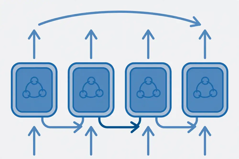
Figure 1: An RNN unfolded through time. Each copy of the cell shares the same weights; the hidden state h flows from step to step, carrying memory forward.
The unfolded view also reveals the architecture's cost: a sequence of 1,000 steps becomes a 1,000-layer network. Deep networks are hard to train, and here the depth is forced on you by the data. Keep that in mind — it is the seed of Chapter 3.
Nothing demystifies the RNN like computing one by hand. Let's use tiny numbers so every step is checkable with a pocket calculator.
Setup. Input dimension 1, hidden dimension 2. Initial hidden state h_0 = [0, 0].
Weights (chosen arbitrarily for illustration):
W_xh = [ 0.5 ] (1×2? No — input dim 1, hidden dim 2, so W_xh is 2×1)
Let me be careful with shapes. If h is a column vector of size 2 and x_t is a scalar, then W_xh must be 2×1 and W_hh must be 2×2. Take:
W_xh = [[ 0.5],
        [-0.3]]

W_hh = [[ 0.8, -0.2],
        [ 0.1,  0.6]]

b_h  = [0, 0]

W_hy = [1.0, -1.0]   (1×2 row vector)
b_y  = 0
Input sequence: x = [1.0, 0.5, -1.0].
Step 1: x_1 = 1.0, h_0 = [0, 0].
z_1 = W_hh·h_0 + W_xh·x_1 + b_h
    = [[0.8,-0.2],[0.1,0.6]]·[0,0] + [[0.5],[-0.3]]·1.0
    = [0.5, -0.3]
h_1 = tanh([0.5, -0.3]) = [0.4621, -0.2913]
y_1 = [1.0, -1.0]·[0.4621, -0.2913] = 0.4621 + 0.2913 = 0.7534
Step 2: x_2 = 0.5.
z_2 = W_hh·h_1 + W_xh·x_2
    = [0.8·0.4621 + (-0.2)·(-0.2913),  0.1·0.4621 + 0.6·(-0.2913)]
      + [0.5·0.5, -0.3·0.5]
    = [0.3697 + 0.0583, 0.0462 - 0.1748] + [0.25, -0.15]
    = [0.4280, -0.1286] + [0.25, -0.15]
    = [0.6780, -0.2786]
h_2 = tanh([0.6780, -0.2786]) = [0.5902, -0.2714]
y_2 = 0.5902 + 0.2714 = 0.8616
Step 3: x_3 = -1.0.
z_3 = W_hh·h_2 + W_xh·x_3
    = [0.8·0.5902 + (-0.2)·(-0.2714),  0.1·0.5902 + 0.6·(-0.2714)]
      + [0.5·(-1.0), -0.3·(-1.0)]
    = [0.4722 + 0.0543, 0.0590 - 0.1628] + [-0.5, 0.3]
    = [0.5265, -0.1038] + [-0.5, 0.3]
    = [0.0265, 0.1962]
h_3 = tanh([0.0265, 0.1962]) = [0.0265, 0.1937]
y_3 = 0.0265 - 0.1937 = -0.1672
Notice what happened: the output at step 3, y_3 = -0.1672, was influenced by x_1 = 1.0 (two steps ago) through the chain h_1 → h_2 → h_3. The memory decayed and transformed as it flowed — that's exactly the dynamics training will shape. Also notice that the whole forward pass is just repeated matrix-vector products: cheap, sequential, and — critically — step t+1 cannot start until step t finishes. That sequential dependency is the RNN's fundamental computational limitation, and it's the reason Transformers (Chapter 9) eventually won on speed.
The architecture above is essentially the Elman network (Jeff Elman, 1990), one of the earliest recurrent designs. Elman's key insight was that the hidden state acts as a context — the network's representation of "where we are in the sequence." He showed that such a network, trained to predict the next word in sentences, spontaneously developed internal representations of grammatical categories (nouns cluster together, verbs cluster together) without ever being told about grammar. That 1990 result is still worth remembering: recurrence forces the network to compress history into a state, and that compression can discover structure you never labeled. When you train an RNN on your own sequence data, ask yourself what structure its hidden state might be discovering — visualizing hidden states (e.g., with t-SNE or PCA) is a legitimate and often illuminating research move.
First, the manual way — an nn.Module that implements the recurrence directly, so you see every operation:
import torch
import torch.nn as nn

class ManualRNN(nn.Module):
    def __init__(self, input_dim, hidden_dim, output_dim):
        super().__init__()
        self.W_xh = nn.Parameter(torch.randn(hidden_dim, input_dim) * 0.5)
        self.W_hh = nn.Parameter(torch.randn(hidden_dim, hidden_dim) * 0.5)
        self.b_h  = nn.Parameter(torch.zeros(hidden_dim))
        self.W_hy = nn.Parameter(torch.randn(output_dim, hidden_dim) * 0.5)
        self.b_y  = nn.Parameter(torch.zeros(output_dim))

    def forward(self, x, h0=None):
        # x: (batch, seq_len, input_dim)
        B, T, _ = x.shape
        h = torch.zeros(B, self.W_hh.shape[0]) if h0 is None else h0
        outputs = []
        for t in range(T):
            z = x[:, t, :] @ self.W_xh.T + h @ self.W_hh.T + self.b_h
            h = torch.tanh(z)
            outputs.append(h @ self.W_hy.T + self.b_y)
        return torch.stack(outputs, dim=1), h   # (B,T,out), final state
And the built-in way, which you will use in practice:
class BuiltinRNN(nn.Module):
    def __init__(self, input_dim, hidden_dim, output_dim, num_layers=1):
        super().__init__()
        self.rnn = nn.RNN(input_dim, hidden_dim, num_layers,
                          batch_first=True, nonlinearity='tanh')
        self.head = nn.Linear(hidden_dim, output_dim)
    def forward(self, x):
        h_seq, h_last = self.rnn(x)      # h_seq: (B,T,H); h_last: (layers,B,H)
        return self.head(h_seq), h_last
The built-in version is faster (fused kernels, cuDNN) and supports stacking layers — num_layers=2 puts a second RNN on top of the first, letting the lower layer learn fast local features and the upper layer learn slower structure. But notice: stacking adds depth in the layer direction, while the sequence still flows through time. Deep-in-time is the hard direction, as Chapter 3 shows.
Let's close with a complete, runnable training example — predicting the next point of a sine wave. It's the "hello world" of sequence modeling, and it works.
import torch, math
import torch.nn as nn
import matplotlib
matplotlib.use("Agg")
import matplotlib.pyplot as plt

torch.manual_seed(7)

# --- Data: sine waves with random phase; input window -> next value ---
def make_data(n_seq=400, T=40):
    X = torch.zeros(n_seq, T, 1); Y = torch.zeros(n_seq, 1)
    for i in range(n_seq):
        phase = torch.rand(1).item() * 2 * math.pi
        t = torch.arange(T + 1).float()
        s = torch.sin(0.3 * t + phase)
        X[i, :, 0] = s[:T]; Y[i, 0] = s[T]
    return X, Y

Xtr, Ytr = make_data(400); Xte, Yte = make_data(100)

model = BuiltinRNN(1, 32, 1)
opt = torch.optim.Adam(model.parameters(), lr=0.01)
lossf = nn.MSELoss()

for epoch in range(300):
    opt.zero_grad()
    preds, _ = model(Xtr)
    loss = lossf(preds[:, -1, :], Ytr)   # many-to-one: use last step's output
    loss.backward(); opt.step()
    if (epoch+1) % 100 == 0:
        print(f"epoch {epoch+1}: train MSE = {loss.item():.5f}")

with torch.no_grad():
    preds, _ = model(Xte)
    print(f"test MSE = {lossf(preds[:, -1, :], Yte).item():.5f}")

# plot one example
with torch.no_grad():
    p, _ = model(Xte[:1])
plt.figure()
plt.plot(Xte[0, :, 0].numpy(), label="input window")
plt.scatter([40], Yte[0].numpy(), c="green", s=60, label="true next")
plt.scatter([40], p[0, -1, 0].numpy(), c="red", s=60, label="predicted next")
plt.legend(); plt.title("Sine-wave next-step prediction")
plt.savefig("/tmp/sine_pred.png")
print("saved /tmp/sine_pred.png")
A 32-unit RNN learns this almost perfectly within a few hundred epochs. The sine wave is smooth and periodic — the hidden state just needs to track phase. Real data is rarely this kind, which is why the rest of the book exists.
For your research: Reproduce this example and then perturb it — add noise, change the frequency mid-sequence, use two superimposed sines. Each perturbation is a tiny research question ("at what noise level does the hidden size need to double?"), and the discipline of changing one thing at a time and measuring is exactly the experimental method Chapter 12 asks you to write up. Reviewers love ablations; this is how you learn to design them.
Three practical details about the hidden state trip up nearly every beginner. Getting them right early saves mysterious bugs later.
1. Initializing h_0. The recurrence needs a starting state. The universal default is the zero vector — simple, and it works because the network quickly learns to overwrite it. An alternative is a learned initial state (a parameter vector optimized during training), which can help when the first few steps matter a lot (short sequences). In PyTorch, nn.RNN defaults to zeros when you don't pass h0; that's fine for almost everything in this book.
2. Resetting state between sequences. This is the classic bug: you train on batches of independent sequences (patient A's ECG, then patient B's ECG) but forget to reset the hidden state between them, so patient B's processing starts from patient A's leftover memory. Within one forward call over a batch, PyTorch handles this — each batch element gets its own state, initialized fresh. The bug appears with truncated BPTT (Chapter 3) or manual loops: if you carry h across chunks, you must detach it (to bound the gradient) but keep it (to preserve memory) within one long sequence — and you must reset it to zeros when a new independent sequence begins. Rule: one independent sequence = one fresh state.
3. Stateful vs. stateless training. In stateless training (the norm), each batch is independent and states reset. In stateful training, you deliberately carry the final state of batch k as the initial state of batch k+1, where batch k+1 continues the same underlying stream (e.g., consecutive chunks of one year's sensor data). Stateful training lets the model learn dependencies longer than your truncation length — at the cost of careful batch bookkeeping (batches must be sequential, shuffling is forbidden). It's a power tool: reach for it when truncated BPTT's k-step limit is the bottleneck and your data is one long stream.
A related design point: stacked RNNs (num_layers=2 or 3). The first layer's hidden states become the second layer's inputs. Intuition: lower layers track fast, local dynamics (oscillations, edges); upper layers track slow, abstract ones (regimes, envelopes). The cost is compute and a longer gradient path in the layer direction — but gating (Chapters 4–5) protects that path too. Two layers is the common sweet spot; beyond three, you usually need residual connections or strong justification.
# Stateful training sketch: batches must be consecutive chunks of one stream
model = BuiltinRNN(1, 32, 1)
h_state = None
stream = torch.randn(10000, 1)          # one long stream
for start in range(0, 10000, 200):      # consecutive, non-shuffled chunks
    chunk = stream[start:start+200].unsqueeze(0)
    preds, h_state = model.rnn(chunk, h_state)
    h_state = h_state.detach()          # bound the gradient...
    # ...but do NOT zero it: memory of the stream persists
    # (zero it only when a genuinely new, independent stream begins)
h_t = tanh(W_hh·h_{t-1} + W_xh·x_t + b_h) is the whole architecture: one transition function, shared across all time steps, with the hidden state as memory.Chapter 2 ended with a warning: unfolding an RNN through time creates a chain as deep as the sequence is long. Now we confront what that depth does to learning. This chapter explains the single most important technical obstacle in the history of recurrent networks — the reason simple RNNs failed on long sequences for years, and the reason the LSTM was invented. If you understand this chapter deeply, the LSTM chapter will feel like the answer to a question you genuinely have, not a bag of tricks to memorize.
Training minimizes a loss L. Gradient descent needs ∂L/∂W for every weight matrix. Consider how the loss at the final step depends on the hidden state at an early step, say h_1, in a T-step sequence. By the chain rule:
∂L/∂h_1 = ∂L/∂h_T · ∂h_T/∂h_{T-1} · ∂h_{T-1}/∂h_{T-2} · ... · ∂h_2/∂h_1
That is a product of T-1 Jacobian matrices. Each Jacobian is:
∂h_t/∂h_{t-1} = diag(tanh'(z_t)) · W_hh
where z_t is the pre-activation and tanh'(z) = 1 - tanh²(z), which lies in (0, 1].
So the gradient flowing backward is multiplied, at every step, by a matrix whose entries are scaled by numbers ≤ 1 and by W_hh. Now comes the decisive observation: multiplying by the same (or similar) matrix many times makes the product's size grow or shrink exponentially, depending on the matrix's largest eigenvalue (its spectral radius — roughly "the factor by which it stretches vectors").
This was proved formally by Bengio, Simard, and Frasconi in 1994: learning long-term dependencies with gradient descent is difficult because the gradient either vanishes or explodes exponentially with the time span. It is not a bug in your code. It is arithmetic.
In practice, vanishing dominates. Two forces push toward it:
What does vanishing mean for learning? Suppose your sequence is a sentence and the loss is at the end: "The keys to the cabinet ___" — the verb should be "are" (agreeing with "keys", 4 steps back). The error signal at the verb must travel back 4 steps to strengthen the connection between "keys" and the hidden state. With vanishing gradients, the signal arrives as dust. The network learns the easy local stuff (word-to-word transitions) and never learns the long-range agreement. It behaves like a student who can only remember the last thing they read.
A worked micro-example makes the arithmetic vivid. Take a scalar RNN: h_t = tanh(w·h_{t-1} + x_t), with w = 0.8. Then ∂h_t/∂h_{t-1} = tanh'(z_t)·0.8 ≤ 0.8. Over 50 steps, the gradient from the end to the start is at most 0.8^50 ≈ 1.4×10⁻⁵. The first input might as well not exist, as far as gradient descent can tell. And with w = 1.2: 1.2^50 ≈ 9,100 — the gradient explodes instead. There is a knife's edge at exactly 1.0, and real weight matrices never sit exactly on it.
Exploding gradients are dramatic — NaN losses, wild oscillations — but they have a simple, effective remedy: gradient clipping. After computing gradients and before applying the update, rescale them if their norm exceeds a threshold:
torch.nn.utils.clip_grad_norm_(model.parameters(), max_norm=1.0)
This doesn't fix the direction problem (the gradient may still point somewhere unhelpful), but it prevents catastrophic updates and is standard practice in every RNN training loop. Think of it as a seatbelt: it doesn't make you a better driver, but it keeps crashes survivable.
Vanishing gradients have no such seatbelt. Clipping can't amplify a signal that has decayed to nothing. The real fix had to be architectural — which is Chapter 4.
Full BPTT on a 10,000-step sequence means a 10,000-deep backward chain: slow, memory-hungry, and vanishing-prone. The standard engineering solution is truncated BPTT: process the sequence in chunks of k steps (say k = 50 or 100), backpropagate only within each chunk, and carry the hidden state forward (detached from the computation graph) between chunks.
# Truncated BPTT sketch
h = None
for chunk in chunks_of(sequence, k=50):
    out, h = model(chunk, h.detach() if h is not None else None)
    loss = criterion(out, targets_for(chunk))
    opt.zero_grad(); loss.backward()
    torch.nn.utils.clip_grad_norm_(model.parameters(), 1.0)
    opt.step()
Truncation limits the gradient's reach to k steps — dependencies longer than k still can't be learned by this mechanism (though the carried hidden state can still transport information forward; it just can't be trained to do so). Choosing k is a real hyperparameter decision: too small and you can't learn real dependencies; too large and you're slow and unstable. In your papers, report k — reviewers in sequence modeling will look for it.
Let's measure gradient magnitudes at different time lags directly, so you see the exponential decay rather than taking it on faith:
import torch
import torch.nn as nn

torch.manual_seed(3)

model = nn.RNN(1, 16, batch_first=True)
head = nn.Linear(16, 1)

T = 60
x = torch.randn(1, T, 1, requires_grad=True)
h, _ = model(x)
out = head(h)
out[0, -1, 0].backward()          # gradient of final output
g = x.grad[0, :, 0].abs()
for lag in [0, 5, 10, 20, 40, 59]:
    print(f"lag {lag:2d} steps back: |d(out_T)/d(x_{{T-lag}})| = {g[T-1-lag]:.2e}")
Typical output shows the gradient shrinking by orders of magnitude as the lag grows — from ~1e-1 at lag 0 down to ~1e-6 or less at lag 40+. Run it, then change the RNN's hidden size or initialization and watch the numbers move. This is the vanishing gradient, measured with your own hands.
Note the subtlety: the gradient we measured flows through the randomly initialized network. Training tries to shape W_hh to fix this, but the shaping signal itself must travel through the vanishing chain — it's trying to lift itself by its bootstraps. That's why the problem is fundamental, not just an initialization issue.
For your research: The vanishing-gradient analysis is a template for how to argue in a paper. "We measured the effective gradient horizon of a vanilla RNN on our dataset (Appendix Fig. X) and found that lags beyond ~30 steps contribute <1% of the gradient norm; since our task requires 100-step dependencies, we adopt an LSTM" — that is a measurement-driven architecture justification. Reviewers accept architectures when the choice is derived from the data's properties, not from fashion. Keep this experiment in your toolkit; you'll reuse it in Chapter 11.
Chapter 3's knife's edge — spectral radius below 1 vanishes, above 1 explodes — raises a practical question: where should W_hh start? Initialization doesn't solve vanishing gradients (training must maintain the dynamics), but a good start keeps early training alive long enough for learning to work.
Xavier/Glorot initialization sets weight variance to keep activation variance stable across layers — designed for feedforward nets, and PyTorch's default for nn.RNN's input weights. For the recurrent matrix specifically, two ideas from the literature matter:
nn.init.orthogonal_(rnn.weight_hh_l0). This is the single most effective cheap trick for training vanilla RNNs on medium-length sequences.Neither trick changes the fundamental story: as training moves W_hh away from its initialization, the exponential dynamics reassert themselves. That's why the field moved to architectural solutions (gating) rather than relying on initialization. But when a reviewer asks "did you try proper initialization for the baseline?", orthogonal init for the vanilla RNN is the answer they want to hear — it makes your "gating beats vanilla" claim honest rather than a strawman.
A final related technique: layer normalization (Ba et al., 2016) applied inside the recurrence re-centers and re-scales the pre-activations at each step, which tames the saturation of tanh (remember: saturated tanh ⇒ near-zero derivatives ⇒ vanishing). nn.LSTM doesn't include it, but several libraries offer LayerNorm variants, and it's a legitimate ablation for a paper's appendix.
Let's derive the vanishing/exploding product explicitly for the simplest possible RNN, so there's no hand-waving left. Scalar state, scalar input:
h_t = tanh(w·h_{t-1} + u·x_t), h_0 = 0
Suppose the loss depends only on the final state: L = ½(h_T − y)². We want ∂L/∂w — how should the recurrent weight change? By the chain rule, w influences L through every time step's state:
∂L/∂w = (h_T − y) · Σ_{k=1..T} [ (∂h_T/∂h_k) · (∂h_k/∂w) ]
Focus on the transport term ∂h_T/∂h_k — how much a nudge to the state at step k matters at step T:
∂h_T/∂h_k = Π_{t=k+1..T} ∂h_t/∂h_{t-1} = Π_{t=k+1..T} tanh'(z_t)·w
There it is: a product of (T−k) terms, each bounded by |w| (since tanh' ≤ 1). If |w| = 0.9 and T−k = 50: the transport is at most 0.9^50 ≈ 0.005 — the gradient from step k barely reaches the loss. If |w| = 1.1: at most 1.1^50 ≈ 117 — amplified a hundredfold. And the direct term ∂h_k/∂w = tanh'(z_k)·h_{k−1} is well-behaved; it's the transport that kills or explodes learning. This derivation is the whole of Bengio et al. (1994) in miniature: the problem isn't the gradient at any one step, it's the multiplicative transport across steps.
Now watch an explosion happen, then get tamed by clipping:
import torch
import torch.nn as nn
torch.manual_seed(0)

# Task: copy the first input's sign to the end of a 40-step sequence (needs long memory)
T = 40
x = torch.randn(300, T, 1); y = (x[:, 0, 0] > 0).long()

class PlainRNN(nn.Module):
    def __init__(self):
        super().__init__()
        self.rnn = nn.RNN(1, 32, batch_first=True)
        self.head = nn.Linear(32, 2)
        # hostile init: large recurrent weights -> explosion-prone
        with torch.no_grad():
            nn.init.normal_(self.rnn.weight_hh_l0, std=1.5)
    def forward(self, x):
        hs, _ = self.rnn(x)
        return self.head(hs[:, -1, :])

def train(clip=None, epochs=60):
    m = PlainRNN(); opt = torch.optim.SGD(m.parameters(), lr=0.05)
    for ep in range(epochs):
        opt.zero_grad()
        loss = nn.CrossEntropyLoss()(m(x), y)
        if torch.isnan(loss).item():
            return f"NaN at epoch {ep} (exploded)"
        loss.backward()
        if clip: nn.utils.clip_grad_norm_(m.parameters(), clip)
        opt.step()
    with torch.no_grad():
        acc = (m(x).argmax(1) == y).float().mean().item()
    return f"finished, train acc = {acc:.3f}"

print("no clipping:  ", train(clip=None))
print("with clipping:", train(clip=1.0))
Typical result: without clipping the loss goes NaN (gradients exploded through the large recurrent weights); with clipping, training survives — though accuracy stays modest, because clipping fixes explosions, not vanishing. The model survives but still can't learn the 40-step dependency well. That gap — survival vs. actual learning — is precisely what gating (Chapter 4) closes.
We now arrive at the architecture that solved the vanishing gradient problem and powered the deep-learning revolution in sequences for two decades: the Long Short-Term Memory network, introduced by Sepp Hochreiter and Jürgen Schmidhuber in 1997. The LSTM is the single most important architecture in this book. Understand it cold — not as a formula to memorize, but as a design whose every part answers the problem of Chapter 3.
A vanilla RNN forces everything — new input and old memory — through the same squashing nonlinearity at every step. The memory gets rewritten, rescaled, and saturated each time, which is exactly what kills gradients.
The LSTM adds a second state vector, the cell state c_t, which acts like a conveyor belt running straight through time. Information can flow along this belt with only linear interactions — elementwise multiplication by gate values — and no repeated squashing. The gradient along the belt is a product of gate values near 1.0, not of squashed derivatives. That is the entire trick, and it is enough.
Around the belt sit three gates — small neural networks that output numbers between 0 and 1 (via sigmoid) and multiply elementwise with the information flowing past:
Gates are the LSTM's genius: instead of the designer fixing the memory dynamics, the network learns its own read/write/erase policy from data, differentiably.
At step t, with input x_t, previous hidden state h_{t-1}, and previous cell state c_{t-1}:
Forget gate — what to discard:
f_t = σ(W_f · [h_{t-1}, x_t] + b_f)
σ is the sigmoid, squashing to (0, 1). f_t = 0 means "erase this memory element completely"; f_t = 1 means "keep it entirely."
Input gate — what new information is worth storing — comes in two parts. First the gate itself:
i_t = σ(W_i · [h_{t-1}, x_t] + b_i)
Then the candidate values to store (this one uses tanh, because candidates should be able to be negative too):
g_t = tanh(W_g · [h_{t-1}, x_t] + b_g)
Cell update — the conveyor belt step:
c_t = f_t ⊙ c_{t-1} + i_t ⊙ g_t
⊙ is elementwise multiplication. Read it as: "keep the fraction f_t of the old memory, and add the fraction i_t of the new candidate." This is the equation that fixes vanishing gradients: ∂c_t/∂c_{t-1} = f_t, and if the forget gate is near 1, the gradient flows backward essentially unchanged. No tanh' squashing in this path at all.
Output gate — what to reveal:
o_t = σ(W_o · [h_{t-1}, x_t] + b_o)
h_t = o_t ⊙ tanh(c_t)
The hidden state is a gated, squashed view of the cell. The cell holds the long-term memory; the hidden state is what the network shows to the outside world (and to the next step's gates) right now.
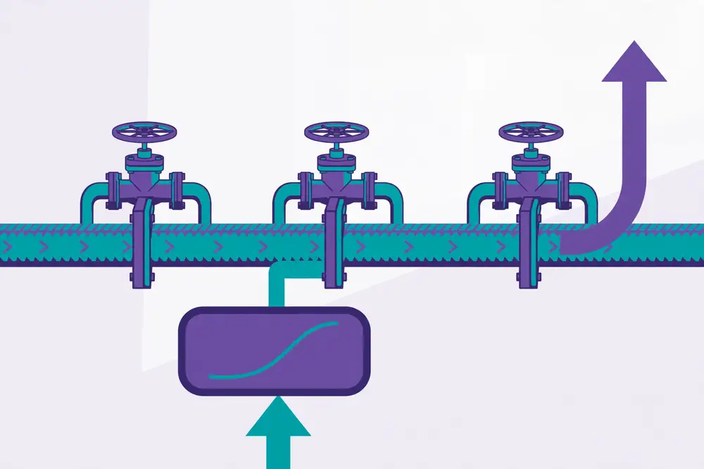
Figure 2: An LSTM cell. The horizontal cell state c is the protected conveyor belt; the three gates (forget, input, output) are learned valves controlling what is erased, written, and read.
Hochreiter and Schmidhuber's original name for the cell-state path was the constant error carousel. Consider the gradient flowing backward along the belt:
∂c_t/∂c_{t-1} = f_t (+ small terms through the gates)
If the network learns f_t ≈ 1 for a memory element, then error flows back through hundreds of steps multiplied by ~1 each time — no exponential decay. The gates are themselves learned, so the network can choose: keep f near 1 for information that must persist (the subject of a sentence, the phase of a slow oscillation), drop f to 0 when context changes (a new paragraph, a regime shift in the data).
This is a profound shift from Chapter 3's knife's edge. In a vanilla RNN, the designer hopes W_hh lands near 1.0 by luck and training. In the LSTM, the default, learnable behavior includes "remember perfectly" — and a standard initialization trick, setting the forget-gate bias b_f to 1.0 (or even 2.0), starts training in the "remember everything" regime so gradients flow from the first epoch.
Let's compute a single step with tiny dimensions so you can verify every number. Hidden/cell size 2, input size 1. Previous states: h_{t-1} = [0.5, -0.2], c_{t-1} = [1.0, 0.5]. Input x_t = [0.8]. Concatenated vector [h_{t-1}, x_t] = [0.5, -0.2, 0.8].
Weights (invented for illustration):
W_f = [[ 0.4, -0.1,  0.2],
       [ 0.3,  0.5, -0.4]],  b_f = [1.0, 1.0]   # forget bias init to 1
W_i = [[ 0.2,  0.3, -0.1],
       [-0.2,  0.4,  0.6]],  b_i = [0.0, 0.0]
W_g = [[ 0.5, -0.3,  0.1],
       [ 0.2,  0.2, -0.5]],  b_g = [0.0, 0.0]
W_o = [[ 0.1,  0.6, -0.2],
       [ 0.4, -0.3,  0.3]],  b_o = [0.0, 0.0]
Forget gate:
z_f = W_f·[0.5,-0.2,0.8] + b_f
    = [0.4·0.5 + (-0.1)·(-0.2) + 0.2·0.8,  0.3·0.5 + 0.5·(-0.2) + (-0.4)·0.8] + [1,1]
    = [0.2 + 0.02 + 0.16,  0.15 - 0.1 - 0.32] + [1, 1]
    = [0.38, -0.27] + [1, 1] = [1.38, 0.73]
f_t = σ([1.38, 0.73]) = [0.799, 0.675]
Interpretation: keep ~80% of memory element 1, ~68% of element 2. (The +1 bias pushes toward remembering.)
Input gate and candidate:
z_i = [0.2·0.5 + 0.3·(-0.2) + (-0.1)·0.8,  (-0.2)·0.5 + 0.4·(-0.2) + 0.6·0.8]
    = [0.1 - 0.06 - 0.08,  -0.1 - 0.08 + 0.48] = [-0.04, 0.30]
i_t = σ([-0.04, 0.30]) = [0.490, 0.574]

z_g = [0.5·0.5 + (-0.3)·(-0.2) + 0.1·0.8,  0.2·0.5 + 0.2·(-0.2) + (-0.5)·0.8]
    = [0.25 + 0.06 + 0.08,  0.1 - 0.04 - 0.4] = [0.39, -0.34]
g_t = tanh([0.39, -0.34]) = [0.371, -0.327]
Cell update:
c_t = f_t ⊙ c_{t-1} + i_t ⊙ g_t
    = [0.799·1.0, 0.675·0.5] + [0.490·0.371, 0.574·(-0.327)]
    = [0.799, 0.3375] + [0.1818, -0.1877]
    = [0.9808, 0.1498]
See the belt in action: element 1 of the memory barely changed (kept 0.799 plus a small addition), because the forget gate stayed open. That near-identity flow is the constant error carousel.
Output gate and hidden state:
z_o = [0.1·0.5 + 0.6·(-0.2) + (-0.2)·0.8,  0.4·0.5 + (-0.3)·(-0.2) + 0.3·0.8]
    = [0.05 - 0.12 - 0.16,  0.2 + 0.06 + 0.24] = [-0.23, 0.50]
o_t = σ([-0.23, 0.50]) = [0.443, 0.622]
h_t = o_t ⊙ tanh(c_t) = [0.443·tanh(0.9808), 0.622·tanh(0.1498)]
    = [0.443·0.7534, 0.622·0.1487] = [0.3338, 0.0925]
That's one full LSTM step, every number checkable. In code you'll never do this, but having done it once, the equations are yours.
import torch
import torch.nn as nn

class ManualLSTMCell(nn.Module):
    def __init__(self, input_dim, hidden_dim):
        super().__init__()
        self.hidden_dim = hidden_dim
        # one combined matrix for all four gates: efficient and standard
        self.W = nn.Parameter(torch.randn(4*hidden_dim, input_dim+hidden_dim) * 0.1)
        self.b = nn.Parameter(torch.zeros(4*hidden_dim))
        with torch.no_grad():                       # forget-bias trick
            self.b[0:hidden_dim].fill_(1.0)

    def forward(self, x_t, state):
        h_prev, c_prev = state
        combined = torch.cat([h_prev, x_t], dim=1)
        gates = combined @ self.W.T + self.b
        f, i, g, o = gates.chunk(4, dim=1)
        f = torch.sigmoid(f); i = torch.sigmoid(i)
        g = torch.tanh(g);    o = torch.sigmoid(o)
        c = f * c_prev + i * g
        h = o * torch.tanh(c)
        return h, c

class ManualLSTM(nn.Module):
    def __init__(self, input_dim, hidden_dim, output_dim):
        super().__init__()
        self.cell = ManualLSTMCell(input_dim, hidden_dim)
        self.head = nn.Linear(hidden_dim, output_dim)
    def forward(self, x, state=None):
        B, T, _ = x.shape
        H = self.cell.hidden_dim
        h = torch.zeros(B, H); c = torch.zeros(B, H)
        if state is not None: h, c = state
        outs = []
        for t in range(T):
            h, c = self.cell(x[:, t, :], (h, c))
            outs.append(self.head(h))
        return torch.stack(outs, dim=1), (h, c)
A good verification exercise: copy weights from nn.LSTM into this cell and check the outputs agree. (Note PyTorch's gate order is i, f, g, o — different from our f, i, g, o ordering — so map the weight blocks carefully.)
Recall Chapter 1's lag-10 task. Let's push the lag to 30 — deep into vanishing territory — and compare:
import torch
import torch.nn as nn
torch.manual_seed(11)

T = 3000; LAG = 30
x = torch.randint(0, 2, (T, 1)).float()
y = torch.zeros(T, 1); y[LAG:] = x[:-LAG]

class SeqModel(nn.Module):
    def __init__(self, kind, h=16):
        super().__init__()
        self.rnn = nn.RNN(1, h, batch_first=True) if kind == "rnn" \
                   else nn.LSTM(1, h, batch_first=True)
        self.head = nn.Linear(h, 1)
    def forward(self, seq):
        h, _ = self.rnn(seq.unsqueeze(0))
        return torch.sigmoid(self.head(h)).squeeze(0)

def train(model, epochs=400):
    opt = torch.optim.Adam(model.parameters(), lr=0.01)
    for _ in range(epochs):
        opt.zero_grad()
        p = model(x)
        loss = nn.BCELoss()(p[LAG:], y[LAG:])
        loss.backward()
        nn.utils.clip_grad_norm_(model.parameters(), 1.0)
        opt.step()
    return model

for kind in ["rnn", "lstm"]:
    m = train(SeqModel(kind))
    with torch.no_grad():
        acc = (((m(x)[LAG:] > 0.5).float() == y[LAG:]).float().mean()).item()
    print(f"{kind.upper():4s} accuracy at lag {LAG}: {acc:.3f}")
The vanilla RNN typically stalls well below the LSTM, which approaches 1.0. Same data, same optimizer — the difference is purely architectural. This is the experiment to show anyone who asks "why not just use a simple RNN?"
The original 1997 LSTM had no forget gate — the cell could only accumulate, never erase, which caused problems on continuous streams (the belt saturated). Gers, Schmidhuber, and Cummins added the forget gate in 2000 ("Learning to forget"), and peephole connections (gates looking at the cell state) followed. The version in this chapter — forget + input + output gates, no peepholes — is the modern standard ("vanilla LSTM" as surveyed by Greff et al., 2017). When you read older papers, check which variant they used; results aren't always comparable across variants.
For your research: The LSTM is a case study in diagnosing before inventing. Hochreiter's 1991 diploma thesis analyzed why gradient-based RNN training fails; the 1997 paper is the fix. If your research proposes a new architecture, reviewers will ask "what specific failure does this fix, and can you demonstrate the failure without your fix?" Build the habit: for every method you propose, first construct the minimal experiment where the baseline fails. That experiment is often the strongest figure in the paper.
Once you train LSTMs, a natural question arises: what did the gates actually learn? Inspecting gate activations is one of the most underused diagnostics in student work, and it's easy:
# Collect average gate activations over a validation sequence
model.eval()
with torch.no_grad():
    # hook into a manual cell, or reimplement the forward with recording
    pass  # see ManualLSTMCell in this chapter: record f, i, o per step
What to look for:
Two variants worth knowing precisely because the literature mentions them:
The meta-lesson: the LSTM is not one fixed object but a family, and the differences between family members are empirical questions. When your paper says "we used an LSTM," specify the variant — future-you trying to reproduce the result will be grateful.
c_t = f_t ⊙ c_{t-1} + i_t ⊙ g_t lets gradients flow back through time multiplied by ~1 (the constant error carousel), defeating vanishing gradients.The LSTM works, but it is heavy: four gate matrices, two state vectors, and a fair amount of computation per step. Researchers soon asked: can we get the same gradient-protecting behavior with fewer moving parts? The answer was the Gated Recurrent Unit (GRU), introduced by Cho et al. in 2014 in the context of neural machine translation. The GRU has become the LSTM's great rival — simpler, faster, and often just as good. This chapter compares them carefully and surveys the wider family of recurrent variants, so you can choose deliberately rather than by habit.
The GRU merges the LSTM's cell state and hidden state into a single state vector h_t, and uses two gates instead of three:
Update gate — how much of the past to keep:
z_t = σ(W_z · [h_{t-1}, x_t] + b_z)
Reset gate — how much of the past to use when computing the new candidate:
r_t = σ(W_r · [h_{t-1}, x_t] + b_r)
Candidate state — the proposed new content, computed with the reset gate throttling the past:
h̃_t = tanh(W_h · [r_t ⊙ h_{t-1}, x_t] + b_h)
Final update — a convex blend of old and new:
h_t = (1 - z_t) ⊙ h_{t-1} + z_t ⊙ h̃_t
Read the last equation carefully — it is the GRU's soul. If z_t ≈ 0, the state passes through unchanged: h_t ≈ h_{t-1}. The gradient ∂h_t/∂h_{t-1} ≈ (1 - z_t) ≈ 1, and we recover the constant-error-carousel behavior that protects against vanishing gradients. If z_t ≈ 1, the state is fully overwritten by the candidate. The reset gate r_t lets the candidate ignore the past when computing something new (useful at sequence boundaries or regime changes).
Compare the parameter counts. For input dimension d and hidden dimension h, an LSTM has 4·(h·(d+h) + h) parameters; a GRU has 3·(h·(d+h) + h) — about 25% fewer. On small datasets that difference matters: fewer parameters mean less overfitting and faster training. Empirically (Chung et al., 2014), GRUs match or beat LSTMs on many tasks, especially with limited data, while LSTMs sometimes win on very long sequences or very large datasets where the extra capacity helps.
There is no theorem that says "use GRU for X, LSTM for Y." But the community has accumulated practical wisdom:
Beyond LSTM and GRU, several variants are worth knowing by name, because you'll meet them in papers:
nn.LSTM(d, h, num_layers=3).Let's make the "25% fewer" claim concrete. Take d = 10 input features, h = 64 hidden units.
LSTM: 4 gates × (h·(d + h) + h) = 4 × (64·74 + 64) = 4 × 4,800 = 19,200 parameters. GRU: 3 gates × (h·(d + h) + h) = 3 × 4,800 = 14,400 parameters. Vanilla RNN: 1 × 4,800 = 4,800 parameters.
At h = 512, d = 128: LSTM ≈ 1.31M, GRU ≈ 0.98M. On a dataset of 5,000 sequences, that 330K-parameter difference is the difference between a model that generalizes and one that memorizes. This is why "simpler wins" is often literally true on small academic datasets.
import torch
import torch.nn as nn
import math
torch.manual_seed(21)

# --- Task: noisy sine with a slow amplitude modulation (needs memory) ---
def make_data(n, T=60):
    X = torch.zeros(n, T, 1); Y = torch.zeros(n, 1)
    for i in range(n):
        phase = torch.rand(1).item()*2*math.pi
        t = torch.arange(T+1).float()
        amp = 1 + 0.5*torch.sin(0.05*t + phase)      # slow envelope
        s = amp*torch.sin(0.4*t + phase) + 0.1*torch.randn(T+1)
        X[i,:,0] = s[:T]; Y[i,0] = s[T]
    return X, Y

Xtr, Ytr = make_data(600); Xte, Yte = make_data(200)

class RNNRegressor(nn.Module):
    def __init__(self, kind, h=32):
        super().__init__()
        self.rnn = {"rnn": nn.RNN, "gru": nn.GRU, "lstm": nn.LSTM}[kind](
            1, h, batch_first=True)
        self.head = nn.Linear(h, 1)
    def forward(self, x):
        hs, _ = self.rnn(x)
        return self.head(hs[:, -1, :])

def run(kind):
    m = RNNRegressor(kind); opt = torch.optim.Adam(m.parameters(), lr=0.01)
    for _ in range(250):
        opt.zero_grad()
        loss = nn.MSELoss()(m(Xtr), Ytr)
        loss.backward(); nn.utils.clip_grad_norm_(m.parameters(), 1.0); opt.step()
    with torch.no_grad():
        te = nn.MSELoss()(m(Xte), Yte).item()
    n_params = sum(p.numel() for p in m.parameters())
    print(f"{kind:5s}: test MSE = {te:.5f}, params = {n_params}")
    return te

for k in ["rnn", "gru", "lstm"]:
    run(k)
Typical results: the vanilla RNN struggles with the amplitude envelope (it can't hold the slow modulation in memory), while GRU and LSTM both do well, with the GRU often slightly ahead on this modestly sized dataset and training ~25% faster per epoch. Change the task — make the envelope slower (0.02 instead of 0.05) — and watch the LSTM's separate cell state start to pull ahead. That sensitivity analysis is a publishable ablation.
One more design decision deserves attention: given a parameter budget, should you make the RNN wider (bigger h) or deeper (more layers)? For sequences, depth buys you hierarchical time: the first layer might track fast oscillations, the second tracks envelopes, the third tracks regime changes. A common recipe: 2 layers × 128 units beats 1 layer × 256 units on complex signals, at similar parameter cost. But each added layer also lengthens the gradient path in the layer direction (mitigated by the same gating) and slows training. Start with 1–2 layers; go deeper only with evidence.
For your research: "We compared LSTM and GRU" is one of the most common — and weakest — sentences in student papers, because it's usually reported without analysis. Make it strong: report parameter counts, training time per epoch, and performance as a function of sequence length or dataset size. "GRU matched LSTM up to 200-step dependencies but degraded beyond 400 steps on our data" is a finding; "LSTM was 2% better" is a footnote. Reviewers reward the finding.
Chapter 5 mentioned encoder-decoder (seq2seq) architectures in passing; they deserve a concrete sketch because they solve the problem class Chapter 1 listed but we haven't built: sequence-to-sequence with different lengths — translation being the canonical example.
The design: an encoder RNN reads the input sequence (say, English words) and compresses it into its final state — the thought vector. A decoder RNN is then initialized with that state and generates the output sequence (French words) one token at a time, each step conditioned on the previous generated token. Training uses teacher forcing: the decoder is fed the true previous token at each step (fast, stable), even though at inference it must feed itself its own predictions (the exposure-bias mismatch from Chapter 7, in its original habitat).
import torch
import torch.nn as nn

class Seq2Seq(nn.Module):
    def __init__(self, vocab_in, vocab_out, emb=32, h=64):
        super().__init__()
        self.enc_emb = nn.Embedding(vocab_in, emb)
        self.encoder = nn.GRU(emb, h, batch_first=True)
        self.dec_emb = nn.Embedding(vocab_out, emb)
        self.decoder = nn.GRU(emb, h, batch_first=True)
        self.head = nn.Linear(h, vocab_out)
    def forward(self, src, tgt):
        # src: (B, Ts) token ids; tgt: (B, Tt) token ids (with <BOS> prepended)
        _, h = self.encoder(self.enc_emb(src))       # thought vector
        dec_in = self.dec_emb(tgt)
        out, _ = self.decoder(dec_in, h)             # decoder seeded with thought vector
        return self.head(out)                        # logits over vocab_out at each step
    @torch.no_grad()
    def generate(self, src, bos_id, eos_id, max_len=30):
        _, h = self.encoder(self.enc_emb(src))
        tok = torch.full((src.size(0), 1), bos_id)
        out_ids = []
        for _ in range(max_len):
            o, h = self.decoder(self.dec_emb(tok), h)
            tok = self.head(o[:, -1, :]).argmax(-1, keepdim=True)
            out_ids.append(tok)
            if (tok == eos_id).all(): break
        return torch.cat(out_ids, dim=1)
The limitation that motivated attention (Chapter 9) is visible here: everything about the input must pass through the single vector h. Sutskever et al. (2014) made this work for translation by reversing the input sequence (a neat trick: it shortens the average dependency distance between corresponding words) and using deep LSTMs — but long sentences still degraded, which is exactly the bottleneck Bahdanau attention removed. When you read modern translation papers, remember: the Transformer decoder is this decoder, with the recurrent step replaced by self-attention and the thought vector replaced by attention over all encoder states.
Chapter 5 introduced bidirectional RNNs briefly; let's make them concrete, because they're the default for labeling tasks and a frequent source of leakage bugs in forecasting.
A bidirectional GRU/LSTM runs two recurrences: one forward (h→_1 … h→_T) and one backward (h←_T … h←_1, reading the sequence reversed). At step t, the representation is the concatenation [h→_t ; h←_t] — what came before and what comes after. In PyTorch it's one flag:
rnn = nn.GRU(input_dim, hidden_dim, batch_first=True, bidirectional=True)
hs, _ = rnn(x)   # hs: (B, T, 2*hidden_dim)
Use bidirectional when the entire sequence is available at decision time: labeling each step of a recorded ECG, tagging words in a finished sentence, classifying a complete activity window. Never use it when step t's output must be produced before step t+1 is observed — forecasting, real-time monitoring, live control. The backward pass is literally reading the future; a bidirectional forecaster is a time machine, and its test scores are fiction. When reviewing others' work, "did they use a bidirectional model for a forecasting task?" is a fast, high-value check.
Where recurrence still wins outright. It's easy to read this book as a history lesson ending in "and then Transformers won." Not so. Recurrence dominates wherever these hold:
The research frontier reflects this: state-space models (SSMs) — the architecture family behind recent efficient sequence models — are essentially linear recurrences with clever parameterization: recurrence's O(T)/O(1) efficiency with better long-range behavior. The pendulum swung from recurrence to attention and is now swinging toward a synthesis. Understanding RNNs deeply is what lets you understand the synthesis.
h_t = (1-z_t)⊙h_{t-1} + z_t⊙h̃_t preserves gradient flow when z_t ≈ 0.You can understand every equation in this book and still fail at sequence modeling, because the most common failures aren't in the model — they're in the data pipeline. This chapter is about the unglamorous work that determines whether your results are real: turning a raw time series into training examples, scaling it without cheating, and splitting it without leaking the future into the past. Get this chapter right and everything downstream is trustworthy; get it wrong and your impressive accuracy is fiction.
Neural networks train on (input, target) pairs. A raw time series is just a sequence of values s_1, s_2, ..., s_N. The sliding window converts it: choose a window length w (how much history the model sees) and a horizon h (how far ahead to predict). Then each training example is:
input:  [s_t, s_{t+1}, ..., s_{t+w-1}]      (w values)
target:  s_{t+w+h-1}                          (the value h steps ahead)
Slide t from 1 to N - w - h + 1, and you get your dataset. Consecutive windows overlap heavily — window t and window t+1 share w-1 values. That's fine; it's how the model sees every possible context.
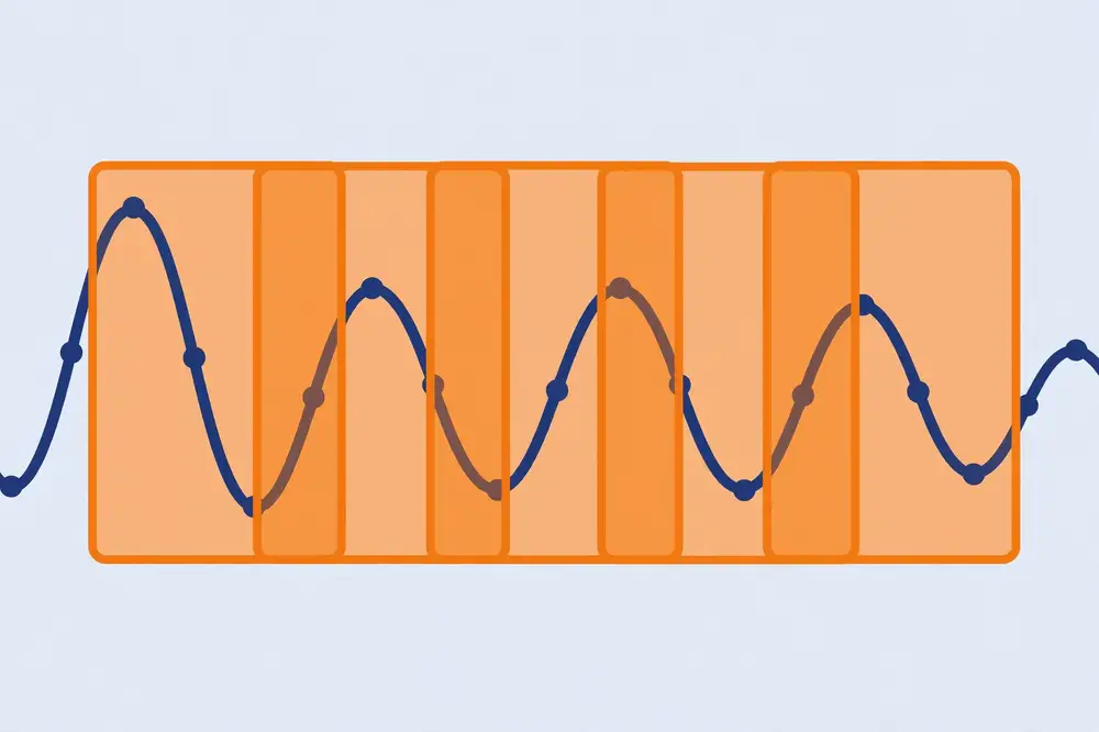
Figure 3: Sliding windows over a time series. Each window of w consecutive values becomes one training input; the window advances one step at a time, and the target is the value h steps ahead of the window's end.
Choosing w is a modeling decision with real consequences:
Multivariate series (multiple sensors/channels) work the same way: each window is a matrix of shape (w, features). Nothing conceptually changes, but scaling (below) becomes per-feature.
Neural networks train best on scaled inputs (roughly zero-mean, unit-variance, or in [0,1]). For time series, the standard choices are:
The critical rule — the one violated in half the student projects I've seen: compute μ, σ, min, max from the training portion only, then apply the same transformation to validation and test. If you compute scaling statistics over the whole dataset, information about the future (the test set's range, its mean) leaks into the training inputs. The model then performs slightly better than it should, and your results are inflated. On some datasets the inflation is small; on volatile ones (finance, energy) it can be dramatic.
import torch

def make_windows(series, w, h=1):
    X, Y = [], []
    for t in range(len(series) - w - h + 1):
        X.append(series[t:t+w])
        Y.append(series[t+w+h-1])
    return torch.stack(X), torch.stack(Y)

# --- The RIGHT way ---
n = len(series)
n_train = int(0.7 * n)
train_raw = series[:n_train]

mu, sigma = train_raw.mean(), train_raw.std()      # statistics from TRAIN only
series_scaled = (series - mu) / sigma              # applied to everything

X, Y = make_windows(series_scaled, w=30, h=1)
# then split X, Y into train/val/test by POSITION (see below)

# --- The WRONG way (do not do this) ---
# mu, sigma = series.mean(), series.std()   # uses future information!
Inverse-transform your errors. If you train on scaled data, your MSE is in scaled units — meaningless to a domain reader. Always convert predictions back (ŷ = ŷ_scaled·σ + μ) and report metrics in original units. Reviewers in applied venues will ask for this.
For i.i.d. data you shuffle and split randomly. For time series, random shuffling is leakage: a test window [s_100..s_129] predicting s_130, trained alongside a training window [s_101..s_130] predicting s_131, means the model has effectively seen the test period during training. The correct split is chronological:
|---- train ----|---- validation ----|---- test ----|
t=1            t_a                  t_b            t=N
One subtlety: because windows overlap, the last training window and the first validation window share values. Purists insert a gap (an embargo period) of w + h steps between splits so no value appears in both. For long series this costs little; for short ones it's a painful but honest trade-off. At minimum, be aware of it and mention your choice in write-ups.
Data leakage — future information sneaking into training — is the #1 reason time-series results don't reproduce. A checklist of classic leaks:
When you review your own pipeline, walk through it asking at each step: "does this number depend on anything after the prediction point?" If yes, it's leakage.
Real time series are messy:
import torch
import torch.nn as nn

torch.manual_seed(5)

# --- Synthetic series: trend + seasonality + noise, with gaps ---
N = 2000
t = torch.arange(N).float()
series = 0.001*t + torch.sin(2*3.14159*t/50) + 0.3*torch.randn(N)
series[500:510] = float('nan'); series[1500:1505] = float('nan')

# 1. Causal imputation: forward fill
mask = torch.isnan(series)
idx = torch.arange(N)
last_valid = torch.maximum.accumulate(torch.where(~mask, idx, torch.zeros(N, dtype=torch.long)))
filled = series[last_valid]
was_missing = mask.float().unsqueeze(1)          # missingness indicator feature

# 2. Chronological split FIRST
n_train, n_val = int(0.6*N), int(0.2*N)
train_raw = filled[:n_train]

# 3. Scale from train only
mu, sigma = train_raw.mean(), train_raw.std()
scaled = (filled - mu) / sigma
features = torch.stack([scaled, was_missing.squeeze()], dim=1)  # (N, 2)

# 4. Windows (w=40, h=1), then split by position with a small embargo gap
W, H, GAP = 40, 1, 5
X, Y = [], []
for i in range(N - W - H + 1):
    X.append(features[i:i+W]); Y.append(scaled[i+W+H-1])
X, Y = torch.stack(X), torch.stack(Y)

n_w = len(X)
i_train = int(0.6*n_w); i_val = int(0.8*n_w)
Xtr, Ytr = X[:i_train], Y[:i_train]
Xva, Yva = X[i_train+GAP:i_val], Y[i_train+GAP:i_val]
Xte, Yte = X[i_val+GAP:], Y[i_val+GAP:]
print(f"train {len(Xtr)}, val {len(Xva)}, test {len(Xte)}")

# 5. Train a GRU forecaster
class Forecaster(nn.Module):
    def __init__(self, h=32):
        super().__init__()
        self.gru = nn.GRU(2, h, batch_first=True)
        self.head = nn.Linear(h, 1)
    def forward(self, x):
        hs, _ = self.gru(x)
        return self.head(hs[:, -1, :]).squeeze(-1)

model = Forecaster(); opt = torch.optim.Adam(model.parameters(), lr=0.01)
for epoch in range(200):
    opt.zero_grad()
    loss = nn.MSELoss()(model(Xtr), Ytr)
    loss.backward(); nn.utils.clip_grad_norm_(model.parameters(), 1.0); opt.step()

# 6. Report in ORIGINAL units
model.eval()
with torch.no_grad():
    pred_scaled = model(Xte)
    pred = pred_scaled*sigma + mu
    true = Yte*sigma + mu
    mae = (pred - true).abs().mean().item()
    rmse = ((pred - true)**2).mean().sqrt().item()
print(f"Test MAE = {mae:.4f}, RMSE = {rmse:.4f} (original units)")
This pipeline — causal imputation, chronological split, train-only scaling, embargo gaps, original-unit metrics — is the template. Copy its structure for every time-series project; adapt the details.
For your research: Data pipelines are under-cited and under-described, which is an opportunity. A short paper or workshop contribution that measures the effect of common leakage mistakes on a public benchmark ("scaling leakage inflates reported accuracy by X% on dataset Y") is genuinely useful to the community and very citable. Reviewers remember authors who made their results more honest.
Classical forecasting theory contributes one idea every deep-learning practitioner should know: stationarity. A stationary series has statistical properties (mean, variance, autocorrelation) that don't drift over time. Neural networks — like most models — learn more easily from stationary data, because the mapping from window to target stays consistent: what "a rise of 2 units" predicts shouldn't depend on whether it's 2020 or 2025.
Many real series are non-stationary: they trend (growing demand), or their variance grows with their level (sales fluctuations proportional to sales). Three standard remedies, applied before windowing:
A related feature-engineering trick: Fourier terms for seasonality. Instead of hoping the RNN discovers weekly periodicity from raw lags, add sin(2πt/7) and cos(2πt/7) (and harmonics) as input features. This is honest feature engineering, not leakage — the calendar is known in advance — and it often improves forecasts dramatically, because you've handed the model the periodic structure explicitly rather than making it rediscover what you already knew. (Hyndman & Athanasopoulos [10] develop these classical ideas fully; they're worth your time even as a deep-learning researcher — the best applied papers blend both traditions.)
Quick diagnostic habit: before modeling any new series, plot it, plot its first differences, and plot its autocorrelation function (ACF). The ACF shows you at which lags the series correlates with itself — that's your data-driven guide to choosing the window length w (Chapter 6) and to predicting which forecasting strategy (Chapter 7) will work.
Forecasting is predicting the future from the past — the most commercially valuable thing sequence models do, from energy load to ICU vital signs to retail demand. Chapter 6 gave you clean windows and honest splits. Now the design question: given a window of history, how do you produce multiple future steps? The answer isn't one method but a family of strategies with different trade-offs, and choosing among them is one of the most consequential decisions in applied sequence modeling.
The simplest task: given the last w values, predict the next value. The model is a function f: R^w → R. Train it on windows (Chapter 6), evaluate with walk-forward validation (Chapter 10). Everything in this chapter builds on this, because multi-step strategies are all ways of extending one-step prediction — or deliberately avoiding that extension.
One-step forecasting is also the right diagnostic: if your model can't predict one step ahead, it has no business predicting ten. Always establish the one-step baseline first.
Suppose you need the next H values (H = 12 hours, 7 days, whatever). Three classical strategies:
1. Recursive (iterative) strategy. Train a one-step model f. To forecast H steps: predict ŷ_{t+1} = f(history), then append ŷ_{t+1} to the history and predict ŷ_{t+2} = f(history + ŷ_{t+1}), and so on. One model, applied H times.
2. Direct strategy. Train H separate models: f_1 predicts 1 step ahead, f_2 predicts 2 steps ahead, ..., f_H predicts H steps ahead. Each model is trained directly on its own horizon.
3. Multi-output (MIMO — multiple input, multiple output) strategy. Train one model with H outputs: f(history) = (ŷ_{t+1}, ..., ŷ_{t+H}). A single forward pass produces the whole horizon.
There is no universal winner. The empirical literature (and the M competitions) suggests: recursive is fine for short H on smooth series; direct often wins at long H where error accumulation kills recursion; MIMO is the modern default in deep learning because one model is operationally simpler and joint outputs are coherent. Your job as a researcher: compare them on your data and report all three. That comparison table is a standard, expected piece of evidence.
The recursive strategy's train/test mismatch deserves a closer look, because fixing it is a real technique. During training with teacher forcing, the model is always fed the true previous values, even when predicting step 5 of a sequence. At inference, it gets its own predictions — which drift. The model never learned to recover from its own errors.
Two remedies:
Let's build all three on a series with both trend and seasonality, forecast H = 12 steps, and compare honestly:
import torch, math
import torch.nn as nn
torch.manual_seed(9)

# --- Data ---
N = 3000
t = torch.arange(N).float()
series = 0.0008*t + torch.sin(2*math.pi*t/48) + 0.5*torch.sin(2*math.pi*t/12) + 0.25*torch.randn(N)

W, H = 48, 12
n_train = int(0.7*(N - W - H + 1))
mu, sigma = series[:n_train + W].mean(), series[:n_train + W].std()
s = (series - mu)/sigma

X, Y = [], []                       # Y: full H-step future for MIMO/direct
for i in range(N - W - H + 1):
    X.append(s[i:i+W]); Y.append(s[i+W:i+W+H])
X, Y = torch.stack(X), torch.stack(Y)
Xtr, Ytr = X[:n_train], Y[:n_train]
Xte, Yte = X[n_train:], Y[n_train:]
print(f"train {len(Xtr)}, test {len(Xte)}")

class GRUHead(nn.Module):
    def __init__(self, out_dim, h=48):
        super().__init__()
        self.gru = nn.GRU(1, h, batch_first=True)
        self.head = nn.Linear(h, out_dim)
    def forward(self, x):
        hs, _ = self.gru(x.unsqueeze(-1))
        return self.head(hs[:, -1, :])

def train_model(model, target, epochs=150):
    opt = torch.optim.Adam(model.parameters(), lr=0.01)
    for _ in range(epochs):
        opt.zero_grad()
        loss = nn.MSELoss()(model(Xtr), target)
        loss.backward(); nn.utils.clip_grad_norm_(model.parameters(), 1.0); opt.step()
    return model

# --- Strategy 1: recursive (one-step model, iterated) ---
one_step = train_model(GRUHead(1), Ytr[:, 0])
with torch.no_grad():
    rec = torch.zeros(len(Xte), H)
    hist = Xte.clone()
    for k in range(H):
        nxt = one_step(hist).squeeze(-1)
        rec[:, k] = nxt
        hist = torch.cat([hist[:, 1:], nxt.unsqueeze(1)], dim=1)

# --- Strategy 2: direct (H models) ---
direct = torch.zeros(len(Xte), H)
for k in range(H):
    m = train_model(GRUHead(1), Ytr[:, k], epochs=150)
    with torch.no_grad(): direct[:, k] = m(Xte).squeeze(-1)

# --- Strategy 3: MIMO (one model, H outputs) ---
mimo = train_model(GRUHead(H), Ytr)
with torch.no_grad(): mimo_pred = mimo(Xte)

def rmse_h(pred):
    return [(((pred[:, k]-Yte[:, k])**2).mean().sqrt()*sigma).item() for k in range(H)]

print("horizon | recursive | direct | mimo   (RMSE, original units)")
for k in range(H):
    r, d, m = rmse_h(rec)[k], rmse_h(direct)[k], rmse_h(mimo_pred)[k]
    print(f"  h={k+1:2d}  |  {r:.4f}  | {d:.4f} | {m:.4f}")
What you'll typically see: recursive starts best (h=1, h=2) then degrades as errors compound; direct stays flat-ish but costs 12 models; MIMO is competitive throughout with one model. The shape of these curves — recursive diverging, direct flat — is the lesson. Plot it: "RMSE vs horizon for three strategies" is exactly the figure reviewers expect in a forecasting paper (Chapter 12).
Everything above predicts a single number per step. But decisions need uncertainty: "demand will be 1,200 units" is less useful than "demand will be 1,200 ± 150 with 90% probability." Two accessible approaches:
You don't need full Bayesian deep learning to be useful. Prediction intervals computed from quantile outputs, evaluated with proper scoring (e.g., mean pinball loss or interval coverage), are a solid, publishable upgrade over point forecasts — and Chapter 10's metrics section covers how to evaluate them.
Real forecasting rarely uses the target series alone. Electricity load depends on temperature; retail demand depends on promotions and holidays. These exogenous variables (covariates) enter as extra input features in each window: X becomes (w, 1 + n_covariates). Two rules: (1) at inference time you must know (or separately forecast) the covariates' future values — calendar features (day of week, holiday flags) are known; temperature must itself be forecast; (2) known-future covariates can also be fed for the horizon steps in MIMO/direct designs. Handling covariates correctly is often where student projects gain their biggest accuracy jump — bigger than any architecture change.
For your research: The strategy comparison (recursive vs direct vs MIMO) is low-hanging, high-value research fruit. Most applied papers pick one strategy without justification. A paper that systematically compares all three across horizons on a new domain dataset, with the RMSE-vs-horizon curves, is a genuine contribution that future researchers in that domain will cite as their justification. It's also the perfect "first paper" scope: one dataset, one clear question, one definitive figure.
Two ideas from the forecasting competitions deserve a place in your toolkit, because they change how you frame problems.
Cross-learning (global models). The traditional approach trains one model per series (one model per store, per sensor). The M4 competition's striking finding (Makridakis et al. [11]) was that global models — one model trained on all series jointly — often win. Why? Each individual series is short and noisy, but the patterns (weekly seasonality, promo effects, trend shapes) repeat across series. A global RNN with series identifiers as features pools statistical strength: it learns the shared patterns from thousands of series and the idiosyncrasies from each one. The catch: the series must be related enough to share structure, and you need per-series scaling (scale each series independently, then feed them jointly). If your problem has many short related series — retail SKUs, sensor fleets, hospital wards — try a global model before building 500 individual ones. It's often both more accurate and operationally simpler (one model to maintain).
Hierarchical forecasting and coherence. Real organizations forecast at multiple aggregation levels: total national demand, regional demand, per-store demand. If you forecast each level independently, the numbers won't add up — the sum of regional forecasts won't equal the national forecast, which destroys trust with decision-makers. Coherent (reconciled) forecasting fixes this: forecast at one level (usually the bottom), then aggregate with a reconciliation method (the "MinT" optimal reconciliation of Hyndman et al. is the modern standard [10]). Deep-learning extensions train the model with a hierarchical loss that penalizes incoherence directly. You may never need this — but the day a stakeholder asks "why don't your forecasts add up?", you'll be glad you know the term.
A final forecasting pitfall worth naming: intermittent demand (spare parts, slow-moving SKUs) — series that are mostly zeros with occasional spikes. Standard MSE-trained RNNs predict near-zero always (minimizing squared error by hugging the majority class). The literature has dedicated methods (Croston's method and its descendants); for deep learning, consider zero-inflated losses or reframing as classification (will there be demand?) plus regression (how much?). Recognizing that your series is intermittent before modeling saves weeks.
Chapter 7 named scheduled sampling as the fix for exposure bias. Here's what it looks like in code, for a multi-step decoder that predicts H steps:
import torch, random

def train_scheduled_sampling(model, Xtr, Ytr, H, epochs=200, p_final=0.5):
    opt = torch.optim.Adam(model.parameters(), lr=0.01)
    for ep in range(epochs):
        # linear schedule: use own predictions more as training progresses
        p = p_final * ep / epochs
        opt.zero_grad()
        B = Xtr.size(0)
        hist = Xtr.clone()
        preds = []
        for k in range(H):
            nxt = model(hist).squeeze(-1)          # one-step model
            preds.append(nxt)
            # scheduled sampling: feed truth or own prediction as next input
            use_pred = (torch.rand(B) < p)
            fed = torch.where(use_pred, nxt.detach(), Ytr[:, k] if k < Ytr.size(1) else nxt.detach())
            hist = torch.cat([hist[:, 1:], fed.unsqueeze(1)], dim=1)
        loss = torch.stack(preds, dim=1).sub(Ytr[:, :H]).pow(2).mean()
        loss.backward(); torch.nn.utils.clip_grad_norm_(model.parameters(), 1.0); opt.step()
    return model
Two practical notes: (1) detaching the fed prediction (nxt.detach()) is essential — otherwise gradients flow through the sampling decisions and training destabilizes; (2) scheduled sampling helps most when the recursive strategy is genuinely needed (variable horizons); if your horizon is fixed, MIMO usually beats scheduled-sampling-enhanced recursion with less fuss. Report which you used — it's a training detail reviewers ask about.
Known-future covariates, worked example. Suppose you're forecasting hourly electricity load and you know the calendar: hour of day, day of week, holiday flags — all known for future hours. Feed them as features for both the history window and the horizon:
# features per step: [load, hour_sin, hour_cos, dow_sin, dow_cos, is_holiday]
# history X: (B, W, 6); future covariates C: (B, H, 5) (no load for future)
# MIMO model variant: encode history, then decode with future covariates
class CovariateForecaster(torch.nn.Module):
    def __init__(self, h=48, H=24):
        super().__init__()
        self.enc = torch.nn.GRU(6, h, batch_first=True)
        self.H = H
        self.dec = torch.nn.GRU(5 + h, h, batch_first=True)
        self.head = torch.nn.Linear(h, 1)
    def forward(self, X_hist, C_future):
        _, h_last = self.enc(X_hist)                       # (1, B, h)
        h_rep = h_last.transpose(0, 1).expand(-1, self.H, -1)  # (B, H, h)
        dec_in = torch.cat([C_future, h_rep], dim=-1)      # future knowns + context
        out, _ = self.dec(dec_in)
        return self.head(out).squeeze(-1)                  # (B, H)
The pattern — encode the past, then decode conditioned on known future information — is extremely general (weather forecasts feeding energy models, scheduled promotions feeding demand models). The rule from Chapter 6 bears repeating: a covariate is only "known-future" if you'd actually know it at forecast time. Temperature forecasts are predictions, not knowns — using actual future temperatures in training is leakage; use the forecasted values (or their historical forecast archives) instead.
Not every sequence problem is forecasting. Often the whole sequence maps to a single label: is this ECG normal or arrhythmic? Is this person walking, running, or sitting? Is this machine bearing healthy or failing? This is sequence classification (many-to-one), and it's where RNNs shine in medicine, wearables, and industrial monitoring. This chapter builds a complete activity-recognition pipeline and an ECG-style classifier, with attention to the evaluation details that make biomedical work trustworthy.
The pattern is simple and reused everywhere:
sequence (T, features) → RNN/GRU/LSTM → final hidden state (H,)
    → Linear(H, classes) → softmax → predicted label
The RNN compresses the whole sequence into its final state; the classifier head reads that summary. Variants: use the mean of all hidden states instead of just the last (mean-pooling — often more robust); use a bidirectional RNN and concatenate both final states (when the full sequence is available); add dropout between the RNN and the head.
Why the final state works: by the end of the sequence, the hidden state has (in principle) integrated everything. In practice, LSTMs/GRUs preserve early information through their gating — which is exactly what Chapters 3–5 were about. If your sequences are very long (thousands of steps), consider mean-pooling or attention-pooling (Chapter 9) instead of relying solely on the last state.
Let's simulate a realistic HAR problem: 3-axis accelerometer data, 128 timesteps per window (about 2.5 seconds at 50 Hz — a standard HAR window), 6 activities. We'll generate synthetic but structurally realistic signals: walking has a strong periodic component at ~2 Hz, running at ~3 Hz with higher amplitude, sitting/standing/lying are near-static with different orientations (gravity on different axes), and stair climbing is periodic but asymmetric.
import torch, math
import torch.nn as nn
torch.manual_seed(42)

ACTIVITIES = ["walking", "upstairs", "downstairs", "sitting", "standing", "lying"]
T, F = 128, 3

def gen_activity(act, n):
    X = torch.zeros(n, T, F)
    t = torch.arange(T).float() / 50.0          # 50 Hz
    for i in range(n):
        noise = 0.08*torch.randn(T, F)
        if act == "walking":
            sig = 0.9*torch.sin(2*math.pi*2.0*t + torch.rand(1)*6.28)
            X[i,:,0] = sig + noise[:,0]; X[i,:,1] = 0.4*sig + noise[:,1]; X[i,:,2] = 9.8 + 0.2*sig + noise[:,2]
        elif act == "upstairs":
            sig = 0.7*torch.sin(2*math.pi*1.6*t + torch.rand(1)*6.28)
            X[i,:,0] = sig + noise[:,0]; X[i,:,1] = 0.5*sig + noise[:,1]; X[i,:,2] = 9.8 + 0.35*torch.abs(sig) + noise[:,2]
        elif act == "downstairs":
            sig = 0.75*torch.sin(2*math.pi*1.8*t + torch.rand(1)*6.28)
            X[i,:,0] = sig + noise[:,0]; X[i,:,1] = 0.45*sig + noise[:,1]; X[i,:,2] = 9.8 - 0.3*torch.abs(sig) + noise[:,2]
        elif act == "sitting":
            X[i,:,0] = noise[:,0]; X[i,:,1] = noise[:,1]; X[i,:,2] = 9.8 + noise[:,2]
        elif act == "standing":
            X[i,:,0] = noise[:,0]; X[i,:,1] = noise[:,1]; X[i,:,2] = 9.8 + noise[:,2]*1.5
        elif act == "lying":
            X[i,:,0] = 9.8 + noise[:,0]; X[i,:,1] = noise[:,1]; X[i,:,2] = noise[:,2]
    return X

# subject-wise split: subjects 0-19 train, 20-23 val, 24-29 test (no subject in two splits!)
def make_split(subjects):
    Xs, ys = [], []
    for s in subjects:
        torch.manual_seed(1000 + s)              # reproducible per subject
        for a, act in enumerate(ACTIVITIES):
            Xs.append(gen_activity(act, 40)); ys += [a]*40
    return torch.cat(Xs), torch.tensor(ys)

Xtr, ytr = make_split(range(20)); Xva, yva = make_split(range(20, 24)); Xte, yte = make_split(range(24, 30))
mu, sd = Xtr.mean((0,1)), Xtr.std((0,1))         # scale from train only
Xtr, Xva, Xte = (Xtr-mu)/sd, (Xva-mu)/sd, (Xte-mu)/sd
print("train/val/test:", Xtr.shape, Xva.shape, Xte.shape)
Note the subject-wise split: no subject appears in more than one split. This is the HAR equivalent of chronological splitting — it's how you prove the model recognizes activities, not individuals. Random splitting here is leakage (the model memorizes subjects' gait quirks). In biomedical ML, subject-wise (or patient-wise) splitting is mandatory, and reviewers will reject papers that split randomly.
The model and training:
class HARNet(nn.Module):
    def __init__(self, h=64):
        super().__init__()
        self.gru = nn.GRU(F, h, num_layers=2, batch_first=True, dropout=0.3)
        self.drop = nn.Dropout(0.3)
        self.head = nn.Linear(h, len(ACTIVITIES))
    def forward(self, x):
        hs, _ = self.gru(x)
        pooled = hs.mean(dim=1)                  # mean-pool over time
        return self.head(self.drop(pooled))

model = HARNet(); opt = torch.optim.Adam(model.parameters(), lr=0.003)
best_va, best_state, patience = 0, None, 0
for epoch in range(200):
    model.train(); opt.zero_grad()
    loss = nn.CrossEntropyLoss()(model(Xtr), ytr)
    loss.backward(); nn.utils.clip_grad_norm_(model.parameters(), 1.0); opt.step()
    model.eval()
    with torch.no_grad():
        va = (model(Xva).argmax(1) == yva).float().mean().item()
    if va > best_va: best_va, best_state, patience = va, {k: v.clone() for k, v in model.state_dict().items()}, 0
    else: patience += 1
    if patience >= 20: break
model.load_state_dict(best_state)
model.eval()
with torch.no_grad():
    pred = model(Xte).argmax(1)
    acc = (pred == yte).float().mean().item()
print(f"Test accuracy: {acc:.3f}")
# confusion matrix
cm = torch.zeros(6, 6, dtype=torch.long)
for t_, p_ in zip(yte, pred): cm[t_, p_] += 1
print("Confusion matrix (rows=true, cols=pred):")
print(cm)
Expect high accuracy on this synthetic data; the instructive part is the confusion matrix. You'll typically see upstairs/downstairs confused with each other (similar periodicity, differing subtly in the vertical channel) and sitting/standing confused (both static, differing only in noise level) — exactly the confusions reported on the real UCI HAR dataset. That correspondence between synthetic and real confusion patterns is worth noting in write-ups: it validates your simulation.
Now a biomedical sketch: detect arrhythmic beats in a synthetic ECG-like signal. Real ECG work uses datasets like MIT-BIH; here we simulate the structure — a repeating QRS-like spike train with occasional premature/ectopic beats — to practice the pipeline:
import torch, math
import torch.nn as nn
torch.manual_seed(7)

T = 200
def gen_ecg(n, anomaly_prob=0.0):
    X = torch.zeros(n, T, 1); y = torch.zeros(n, dtype=torch.long)
    t = torch.arange(T).float()
    for i in range(n):
        beat_every = 40
        sig = torch.zeros(T)
        pos = 10
        abnormal = torch.rand(1).item() < anomaly_prob
        while pos < T - 10:
            width = 6 if not abnormal or torch.rand(1).item() > 0.3 else 14  # wide beat
            amp = 1.0 if not abnormal or torch.rand(1).item() > 0.3 else 0.5
            sig += amp*torch.exp(-((t-pos)**2)/(2*(width/2.35)**2))
            pos += beat_every + int(torch.randn(1).item()*2)
        X[i,:,0] = sig + 0.05*torch.randn(T)
        y[i] = 1 if abnormal else 0
    return X, y

Xtr, ytr = gen_ecg(800, 0.5); Xte, yte = gen_ecg(200, 0.5)
mu, sd = Xtr.mean(), Xtr.std(); Xtr, Xte = (Xtr-mu)/sd, (Xte-mu)/sd

class ECGNet(nn.Module):
    def __init__(self, h=48):
        super().__init__()
        self.lstm = nn.LSTM(1, h, batch_first=True, bidirectional=True)
        self.head = nn.Linear(2*h, 2)
    def forward(self, x):
        hs, _ = self.lstm(x)
        return self.head(hs[:, -1, :])           # last step, both directions

model = ECGNet(); opt = torch.optim.Adam(model.parameters(), lr=0.003)
for epoch in range(120):
    model.train(); opt.zero_grad()
    loss = nn.CrossEntropyLoss()(model(Xtr), ytr)
    loss.backward(); nn.utils.clip_grad_norm_(model.parameters(), 1.0); opt.step()

model.eval()
with torch.no_grad():
    p = model(Xte).argmax(1)
    acc = (p == yte).float().mean().item()
    tp = ((p==1)&(yte==1)).sum().item(); fp = ((p==1)&(yte==0)).sum().item()
    fn = ((p==0)&(yte==1)).sum().item()
    prec = tp/(tp+fp+1e-9); rec = tp/(tp+fn+1e-9)
print(f"acc={acc:.3f}  precision={prec:.3f}  recall={rec:.3f}  F1={2*prec*rec/(prec+rec+1e-9):.3f}")
For medical tasks, accuracy alone is never enough — report precision, recall, and F1, because the costs of errors are asymmetric (missing an arrhythmia vs. a false alarm). Also note we used a bidirectional LSTM here: for beat classification the whole strip is available at inference, so future context is legitimate (not leakage — this isn't forecasting).
weight= in CrossEntropyLoss), oversampling, or focal loss — and always report per-class metrics, not just overall accuracy.pack_padded_sequence so the RNN ignores padding; or truncate/pad to a fixed window as we did. In papers, state your choice.For your research: Sequence classification on sensor/biomedical data is one of the most accessible paths to a first publication: the datasets are public (UCI HAR, MIT-BIH, PAMAP2), the baselines are clear, and the evaluation standards are well understood. A strong student contribution: take a dataset where the leaderboard uses hand-crafted features + SVM/random forest, and show a simple GRU/LSTM with careful splitting and augmentation matching or beating it — with ablations showing which design choice mattered. Novelty doesn't have to mean a new architecture; rigorous application to an underexplored dataset or population is novelty too.
Classification assigns one label per sequence; many real problems need one label per time step — the many-to-many (aligned) shape from Chapter 1. Examples: sleep-stage scoring (each 30-second EEG epoch gets a stage: awake, REM, N1–N3), part-of-speech tagging (each word gets a grammatical tag), human-activity segmentation (label every timestep of a continuous recording, not just pre-cut windows).
The architecture is a small change from classification: instead of pooling, put the classifier head on every hidden state:
class SequenceLabeler(nn.Module):
    def __init__(self, in_dim, h=64, n_classes=5):
        super().__init__()
        # bidirectional: label at step t can use past AND future
        self.rnn = nn.GRU(in_dim, h, batch_first=True, bidirectional=True)
        self.head = nn.Linear(2*h, n_classes)
    def forward(self, x):
        hs, _ = self.rnn(x)          # (B, T, 2h): a state per step
        return self.head(hs)         # (B, T, classes): logits per step
# loss: nn.CrossEntropyLoss()(logits.transpose(1,2), labels)  # labels: (B, T)
Bidirectionality is the norm here (the full sequence exists at inference), and the loss is computed per step, usually averaged. Two practical issues dominate:
When input and output sequences aren't aligned step-to-step (speech: audio frames vs. characters, where you don't know which frames correspond to which letters), the alignment problem needs CTC (Connectionist Temporal Classification, Graves et al., 2006): the network outputs a label (or "blank") per input step, and the loss marginalizes over all alignments consistent with the target sequence. CTC powered a generation of speech recognizers. You don't need its full machinery for most sensor work — but knowing its name lets you recognize alignment problems when you meet them, instead of forcing them into a per-step-labeling mold that doesn't fit.
Real sequences vary in length — one patient's ECG strip is 8 seconds, another's is 30. Neural networks train in rectangular batches, so we pad shorter sequences (usually with zeros) to the batch's max length. But the RNN must not learn from padding: zeros fed as inputs pollute the hidden state, and mean-pooling over padded steps dilutes the signal.
PyTorch's answer is packing: pack_padded_sequence tells the RNN the true length of each sequence, so it stops processing at the right step and the final state genuinely reflects the last real input:
import torch
import torch.nn as nn
from torch.nn.utils.rnn import pack_padded_sequence, pad_packed_sequence

# batch of 3 sequences, true lengths 5, 3, 4, padded to 5
X = torch.randn(3, 5, 8)
lengths = torch.tensor([5, 3, 4])

# pack_padded_sequence needs lengths in descending order (or enforce_sorted=False)
order = torch.argsort(lengths, descending=True)
Xo, lo = X[order], lengths[order]

rnn = nn.GRU(8, 16, batch_first=True)
packed = pack_padded_sequence(Xo, lo.tolist(), batch_first=True)
_, h_last = rnn(packed)          # h_last: (1, 3, 16) — true final states, no padding pollution
h_last = h_last.squeeze(0)[torch.argsort(order)]  # restore original order

# For per-step outputs with masking (e.g., attention or mean-pool over real steps only):
out_packed, _ = rnn(packed)
hs, _ = pad_packed_sequence(out_packed, batch_first=True)  # (3, 5, 16), padded tail = 0
hs = hs[torch.argsort(order)]
mask = torch.arange(5).unsqueeze(0) < lengths.unsqueeze(1)  # (3, 5) True for real steps
pooled = (hs * mask.unsqueeze(-1)).sum(1) / lengths.unsqueeze(-1).float()
Three rules to remember: (1) always pack (or mask) — never let padding silently enter the loss or the pooling; (2) keep a lengths tensor alongside every batch — your dataloader should return (padded_batch, lengths, labels); (3) in your paper's method section, state the padding strategy and max length — reviewers checking reproducibility need it. A common alternative for very long sequences is truncation to a fixed window (losing the tail) — state that choice too, with justification.
So far, information flows through sequences one step at a time, squeezed through a fixed-size hidden state. That squeezing is a bottleneck: to translate a 50-word sentence, the encoder must cram all 50 words' meaning into one vector, and the decoder must unpack it. In 2014–2015, Bahdanau, Cho, and Bengio asked a liberating question: what if the decoder could look back at all the encoder's states and choose which ones matter for each output word? The answer — attention — didn't just fix translation; it became the most important idea in modern deep learning and the direct ancestor of the Transformer. This chapter teaches attention as the natural next step after RNNs.
In encoder-decoder RNNs (Chapter 5), the encoder reads the input sequence and hands the decoder a single final state — the "thought vector." For short sequences this works. For long ones, performance collapses: the fixed-size vector can't hold a long sentence's content, and the decoder has no way to recover what was lost. It's like being asked to translate a paragraph after hearing it once, with no notes allowed.
Attention gives the decoder notes. Instead of one vector, the encoder keeps all its hidden states h_1, ..., h_T. At each decoding step, the decoder computes a score for how relevant each encoder state is to the current output, turns the scores into weights (softmax), and takes a weighted average — the context vector. The decoder then generates the next output from the context vector plus its own state. Different output steps attend to different input parts: when generating the French word for "cat," the decoder attends to the encoder state for "cat."
Let the encoder states be h_1, ..., h_T (each a vector), and let s_{t-1} be the decoder's state before generating output step t.
Scores — how well does encoder state j match what the decoder needs now? The original (Bahdanau) formulation uses a small learned network:
e_{t,j} = vᵀ · tanh(W·s_{t-1} + U·h_j)
Weights — normalize the scores into a probability distribution over input positions:
α_{t,j} = exp(e_{t,j}) / Σ_k exp(e_{t,k})
Context — the weighted average, the decoder's "notes" for this step:
c_t = Σ_j α_{t,j} · h_j
The decoder then computes its new state and output from s_{t-1}, c_t, and the previous output. That's it. Three equations, and the bottleneck is gone: the decoder has direct, differentiable access to every input position, with gradients flowing straight back through the weighted average — no long chain, no vanishing.
Three consequences made attention revolutionary:
For time-series researchers, attention over RNN states is the pragmatic middle ground: keep the RNN's sequential inductive bias (useful for smooth physical signals) and add attention for long-range access and interpretability.
Tiny example. Encoder states (2-D) for a 4-step input:
h_1 = [1.0, 0.0], h_2 = [0.0, 1.0], h_3 = [1.0, 1.0], h_4 = [0.5, 0.5]
Decoder state s = [1.0, 0.0]. Use simplified dot-product scores e_j = s·h_j (the real Bahdanau score is a learned network; dot-product is its efficient cousin, used in Transformers):
e_1 = 1.0·1.0 + 0.0·0.0 = 1.0
e_2 = 1.0·0.0 + 0.0·1.0 = 0.0
e_3 = 1.0·1.0 + 0.0·1.0 = 1.0
e_4 = 1.0·0.5 + 0.0·0.5 = 0.5
Softmax: exp([1.0, 0.0, 1.0, 0.5]) = [2.718, 1.0, 2.718, 1.649]; sum = 8.085.
α = [0.336, 0.124, 0.336, 0.204]
Context vector:
c = 0.336·[1.0,0.0] + 0.124·[0.0,1.0] + 0.336·[1.0,1.0] + 0.204·[0.5,0.5]
  = [0.336 + 0 + 0.336 + 0.102,  0 + 0.124 + 0.336 + 0.102]
  = [0.774, 0.562]
The decoder focused mostly on steps 1 and 3 (the ones most similar to its current state) — exactly the "look up what's relevant" behavior. Now imagine s changing each decoding step: the focus shifts, producing the alignment patterns you see in translation heatmaps.
Let's add attention to a forecaster and visualize where it looks — the interpretability payoff:
import torch, math
import torch.nn as nn
torch.manual_seed(17)

# --- Series with two rhythms: fast daily + slow weekly ---
N = 2500
t = torch.arange(N).float()
series = torch.sin(2*math.pi*t/24) + 0.6*torch.sin(2*math.pi*t/168) + 0.2*torch.randn(N)

W = 72
mu, sd = series[:1500].mean(), series[:1500].std()
s = (series - mu)/sd
X = torch.stack([s[i:i+W] for i in range(N - W)])
Y = s[W:]
Xtr, Ytr = X[:1500], Y[:1500]
Xte, Yte = X[1500:], Y[1500:]

class AttnForecaster(nn.Module):
    def __init__(self, h=48):
        super().__init__()
        self.enc = nn.GRU(1, h, batch_first=True)
        # Bahdanau-style scoring: v^T tanh(W s + U h_j)
        self.Ws = nn.Linear(h, h, bias=False)
        self.Us = nn.Linear(h, h, bias=False)
        self.v  = nn.Linear(h, 1, bias=False)
        self.head = nn.Linear(2*h, 1)
    def forward(self, x, return_attn=False):
        hs, _ = self.enc(x.unsqueeze(-1))        # (B, W, h)
        s_last = hs[:, -1, :]                    # decoder "state": last encoder state
        scores = self.v(torch.tanh(self.Ws(s_last).unsqueeze(1) + self.Us(hs))).squeeze(-1)
        alpha = torch.softmax(scores, dim=1)     # (B, W)
        context = (alpha.unsqueeze(-1) * hs).sum(dim=1)
        out = self.head(torch.cat([s_last, context], dim=1)).squeeze(-1)
        return (out, alpha) if return_attn else out

model = AttnForecaster(); opt = torch.optim.Adam(model.parameters(), lr=0.01)
for epoch in range(150):
    opt.zero_grad()
    loss = nn.MSELoss()(model(Xtr), Ytr)
    loss.backward(); nn.utils.clip_grad_norm_(model.parameters(), 1.0); opt.step()

model.eval()
with torch.no_grad():
    pred, alpha = model(Xte[:8], return_attn=True)
    print(f"test RMSE (orig units): {(((model(Xte)-Yte)**2).mean().sqrt()*sd).item():.4f}")
    # where did it look? average attention over 8 examples, by lag
    avg = alpha.mean(0)
    peaks = torch.topk(avg, 5)
    print("most-attended lags (steps back from forecast point):",
          [W-1-i for i in peaks.indices.tolist()])
On this data, the top attended lags usually cluster near 24 and 48 steps back — the daily rhythm — and sometimes near 168 (weekly). The model rediscovers the series' periodicities in its attention weights. That is a beautiful result to show in a paper: domain knowledge (the series has daily/weekly cycles) emerging from the model's learned behavior, confirming both the model and your understanding.
Once you have attention, ask: do we still need the recurrence? The RNN encoder's job was to build the h_j states — but attention itself can build contextualized representations: let every position attend to every other position (self-attention), stack several such layers, and add position information (since attention is order-blind, you must inject position via positional encodings). The result is the Transformer: no recurrence, fully parallel, and — with enough data — more powerful.
The practical consequence for your work: for long sequences with abundant data, try Transformers; for modest data or strong sequential structure (physics, physiology), RNNs + attention remain competitive and cheaper. The Learning Dashboard (Appendix A) compares them head-to-head. And note the irony: the RNN's sequential bottleneck (Chapter 2) is precisely what attention routes around — understanding RNNs first makes the Transformer's design choices legible rather than magical.
For your research: Attention heatmaps are among the most persuasive figures in sequence-modeling papers — but also among the most overclaimed. If you show one, accompany it with a quantitative check: e.g., "attention mass on the known QRS region correlates r=0.8 with the model's confidence," or an ablation where masking the attended regions degrades performance more than masking random regions. Reviewers increasingly demand this; the "attention is not explanation" debate means pretty heatmaps alone no longer suffice.
Chapter 9 used single-head Bahdanau attention. The Transformer (Vaswani et al. [9]) refined attention into two ideas worth understanding even if you never build a full Transformer — because "Transformer encoder" layers are now a standard drop-in alternative to RNN layers in sequence pipelines.
Scaled dot-product attention. Instead of the learned Bahdanau scorer, use dot products — but scaled:
Attention(Q, K, V) = softmax(Q·Kᵀ / √d) · V
Q (queries), K (keys), V (values) are linear projections of the input states. The √d scaling is not cosmetic: without it, dot products grow with dimension d, the softmax saturates, and gradients die — the same saturation story as tanh, in a new costume. In self-attention, Q, K, V all come from the same sequence: every position attends to every position, building context-aware representations in parallel.
Multiple heads. One attention distribution can only express one notion of relevance ("similar words"). Multi-head attention runs h independent attention mechanisms in parallel (each with its own Q/K/V projections, at dimension d/h) and concatenates the results. Empirically, different heads specialize: one tracks local neighbors, another tracks syntactic relations, another tracks long-range coreference. It's the attention equivalent of having multiple convolutional filters — representational diversity from parallelism.
Positional encodings. Attention is order-blind: permute the input and the output permutes identically (it's permutation-equivariant). But order matters in sequences! The Transformer therefore adds position information to each input: the original paper used fixed sinusoidal encodings (sines/cosines at geometrically increasing wavelengths — a clever choice because relative offsets become linear transformations), while modern variants learn positional embeddings. This is the one place the Transformer is weaker than the RNN by design: recurrence gets order for free; attention must be told.
For your work, the practical takeaway: a "Transformer encoder" (nn.TransformerEncoder in PyTorch) can replace the GRU/LSTM in the classifiers and forecasters of Chapters 7–8 as a drop-in experiment. On small datasets it often loses to the GRU (less inductive bias, more data hunger); on large ones it wins. That comparison — same pipeline, RNN vs. Transformer encoder, with data-size ablations — is itself a publishable empirical study on many domain datasets.
Attention isn't only for seq2seq — its simplest use is attention pooling for classification: instead of mean-pooling all hidden states equally, learn which timesteps deserve weight. A violent cough in an audio clip, the anomalous beat in an ECG strip — the model learns to focus on the informative moments.
class AttnPoolClassifier(nn.Module):
    def __init__(self, in_dim, h=64, n_classes=6):
        super().__init__()
        self.rnn = nn.GRU(in_dim, h, batch_first=True, bidirectional=True)
        self.attn = nn.Linear(2*h, 1)      # scores each timestep
        self.head = nn.Linear(2*h, n_classes)
    def forward(self, x, return_attn=False):
        hs, _ = self.rnn(x)                          # (B, T, 2h)
        scores = self.attn(torch.tanh(hs)).squeeze(-1)  # (B, T)
        alpha = torch.softmax(scores, dim=1)
        context = (alpha.unsqueeze(-1) * hs).sum(dim=1) # (B, 2h)
        out = self.head(context)
        return (out, alpha) if return_attn else out
Compared with mean-pooling (Chapter 8), attention pooling usually helps when the discriminative signal is localized — a brief anomaly in a long normal recording. When the signal is diffuse (overall rhythm, average intensity), mean-pooling is often just as good and simpler. That's an ablation worth running: same backbone, mean-pool vs. attention-pool, reported side by side.
The interpretability payoff is immediate: plot α over time for a test example and you see where the model looked. On the synthetic ECG task from Chapter 8, the attention peaks land on the wide/ectopic beats — the model rediscovers the clinically relevant morphology without being told. Two caveats from the literature, to keep you honest: (1) attention weights are plausible explanations, not faithful ones — different weight distributions can produce the same output, so validate with the masking ablations from Chapter 9's research box; (2) with small datasets, the attention layer itself can overfit to spurious timesteps — regularize it (dropout on the scores) and check that attended regions are stable across seeds before claiming a finding.
A model is only as good as its evaluation. In time-series work, evaluation has more traps than modeling: the wrong split, the wrong metric, or the wrong baseline can make a useless model look state-of-the-art — and these mistakes survive peer review more often than you'd hope. This chapter gives you the evaluation discipline that separates trustworthy work from impressive-looking fiction.
A forecaster deployed in the real world is retrained (or at least re-run) as new data arrives: train on January–June, forecast July; then train on January–July, forecast August; and so on. Walk-forward validation (also called rolling-origin evaluation) replicates this: it measures performance across many "as-of" dates instead of one lucky test split.
The procedure:
Fold 1: train [1..t1]          → test (t1..t2]
Fold 2: train [1..t2]          → test (t2..t3]
Fold 3: train [1..t3]          → test (t3..t4]
...average the test scores...
Two variants: expanding window (train set grows each fold — uses all history, standard) and sliding window (train set is a fixed-length recent block — appropriate when old data is stale, e.g., regime changes). Retraining from scratch each fold is expensive; in practice, many researchers train once per fold but warm-start from the previous fold's weights. Report whichever you did.
Why not a single train/test split? Because a single split measures performance on one future period. If that period was unusually calm or volatile, your score is misleading. Walk-forward averages over many periods and also reveals stability: a model great in 3 folds and terrible in 2 is telling you something important.
import torch
import torch.nn as nn

def walk_forward(series, make_model, W=48, H=1, n_folds=5, test_len=200, epochs=80):
    s = (series - series[:1000].mean()) / series[:1000].std()  # scale from initial block
    fold_rmses = []
    t_end = 1000
    for fold in range(n_folds):
        tr_end, te_end = t_end, t_end + test_len
        Xtr = torch.stack([s[i:i+W] for i in range(tr_end - W)])
        Ytr = s[W:tr_end]
        Xte = torch.stack([s[i:i+W] for i in range(tr_end, te_end - W)])
        Yte = s[tr_end+W:te_end]
        model = make_model(); opt = torch.optim.Adam(model.parameters(), lr=0.01)
        for _ in range(epochs):
            opt.zero_grad()
            loss = nn.MSELoss()(model(Xtr).squeeze(-1), Ytr)
            loss.backward(); opt.step()
        with torch.no_grad():
            rmse = (((model(Xte).squeeze(-1) - Yte)**2).mean().sqrt()).item()
        fold_rmses.append(rmse); print(f"fold {fold+1}: RMSE = {rmse:.4f}")
        t_end = te_end
    print(f"mean ± std: {sum(fold_rmses)/n_folds:.4f} ± {torch.tensor(fold_rmses).std().item():.4f}")
    return fold_rmses

class TinyGRU(nn.Module):
    def __init__(self, h=32):
        super().__init__()
        self.gru = nn.GRU(1, h, batch_first=True); self.head = nn.Linear(h, 1)
    def forward(self, x):
        hs, _ = self.gru(x.unsqueeze(-1)); return self.head(hs[:, -1, :])
Different metrics punish different mistakes. Know what yours measures:
The naive baselines you must beat. Every forecasting paper must compare against:
If your deep model can't beat seasonal naive, you don't have a deep learning result — you have a deep learning expense. Report these baselines in every results table. Reviewers check.
"Our model got RMSE 3.21 vs baseline 3.34" — is that a real improvement or noise? With walk-forward folds, you have paired samples (both models scored on the same folds), so use a paired test:
At minimum, report variability (std across folds), not just the mean. A "win" of 2% with fold-std of 5% is not a win.
For your research: Evaluation rigor is a differentiator. Many published sequence-modeling papers fail items on this checklist. A paper whose main contribution is "we evaluated existing methods properly on dataset X and found the rankings change" — with walk-forward validation, proper baselines, and significance tests — is publishable and heavily cited, because everyone building on dataset X needs your numbers. Rigor is a research contribution, not just hygiene.
Walk-forward validation is sometimes called backtesting (the term comes from finance). A few pitfalls specific to backtesting deserve explicit warning, because they're subtler than the Chapter 6 leakage list:
The Diebold-Mariano test, briefly: you have two models' forecast errors over the same test periods. Define the loss differential d_t = L(e_A,t) − L(e_B,t) (e.g., squared errors). Under the null hypothesis of equal accuracy, the mean of d_t is zero. The DM statistic is essentially the mean differential divided by its standard error (with a correction for autocorrelation in multi-step forecasts, since overlapping horizons create correlated errors). A significant statistic means one model genuinely wins. In practice: use the dieboldmariano implementations in standard stats libraries, apply it to walk-forward fold errors, and report the p-value alongside the headline numbers. It's a small addition that converts "3.21 vs 3.34" from a shrug into a claim.
One more honest practice: report the number of folds each model won, not just the average. "GRU won 4 of 5 folds" communicates robustness in a way that a bare mean never can — and it occasionally reveals that a "winning" average came from one lucky fold.
Let's put the whole chapter together in one runnable script: walk-forward evaluation, three baselines plus a GRU, MASE, fold-win counts, and a simple paired significance test (a sign test over folds — no extra dependencies needed).
import torch, math
import torch.nn as nn
torch.manual_seed(99)

# --- Data: trend + daily seasonality + noise ---
N = 4000
t = torch.arange(N).float()
series = 0.0006*t + 2.0*torch.sin(2*math.pi*t/24) + 0.4*torch.randn(N)
SEASON = 24

def mase(err_model, y_true, y_train):
    # scale-free: MAE relative to in-sample naive MAE
    naive_mae = (y_train[1:] - y_train[:-1]).abs().mean()
    return (err_model.abs().mean() / naive_mae).item()

def sign_test(wins_a, n):
    # two-sided binomial p-value under H0: P(win)=0.5 (implemented directly)
    from math import comb
    k = min(wins_a, n - wins_a)
    return sum(comb(n, i) for i in range(k + 1)) * 2 / 2**n

class GRU1(nn.Module):
    def __init__(self, h=32):
        super().__init__()
        self.gru = nn.GRU(1, h, batch_first=True); self.head = nn.Linear(h, 1)
    def forward(self, x):
        hs, _ = self.gru(x.unsqueeze(-1)); return self.head(hs[:, -1, :]).squeeze(-1)

W, FOLDS, TEST = 72, 5, 300
results = {"naive": [], "seas_naive": [], "ma": [], "gru": []}
t0 = 1200
for f in range(FOLDS):
    tr = series[:t0]; te = series[t0:t0+TEST]
    mu, sd = tr.mean(), tr.std()
    str_, ste = (tr-mu)/sd, (te-mu)/sd
    # windows over train
    Xtr = torch.stack([str_[i:i+W] for i in range(len(str_)-W)])
    Ytr = str_[W:]
    # test windows: each test point predicted from the W preceding (true) values
    full = torch.cat([str_[-W:], ste])
    preds = {}
    preds["naive"]      = full[W-1:-1]                       # persistence
    preds["seas_naive"] = full[W-SEASON:-SEASON]             # same hour yesterday
    ma_hist = full[:W].clone()
    ma_preds = []
    for k in range(TEST):
        ma_preds.append(ma_hist[-SEASON:].mean())
        ma_hist = torch.cat([ma_hist, full[W+k:W+k+1]])
    preds["ma"] = torch.stack(ma_preds)
    # GRU
    m = GRU1(); opt = torch.optim.Adam(m.parameters(), lr=0.01)
    for _ in range(120):
        opt.zero_grad(); l = nn.MSELoss()(m(Xtr), Ytr)
        l.backward(); nn.utils.clip_grad_norm_(m.parameters(), 1.0); opt.step()
    with torch.no_grad():
        Xte = torch.stack([full[i:i+W] for i in range(TEST)])
        preds["gru"] = m(Xte)
    truth = ste[:TEST]
    for name, p in preds.items():
        err = (p - truth)*sd                                 # back to original units
        results[name].append((err.abs().mean().item(), mase(err, truth, tr)))
    t0 += TEST

print(f"{'model':12s} {'MAE':>8s} {'MASE':>7s}  (mean over {FOLDS} folds)")
for name, vals in results.items():
    mae = sum(v[0] for v in vals)/FOLDS; ms = sum(v[1] for v in vals)/FOLDS
    print(f"{name:12s} {mae:8.4f} {ms:7.3f}")
# fold wins + significance: GRU vs seasonal naive on MAE
wins = sum(1 for f in range(FOLDS) if results["gru"][f][0] < results["seas_naive"][f][0])
print(f"GRU beat seasonal-naive in {wins}/{FOLDS} folds; sign-test p = {sign_test(wins, FOLDS):.3f}")
What this script gives you — and what your papers should always include: (1) baselines that were genuinely hard to beat (seasonal naive is strong on this data); (2) MASE so the numbers are comparable across datasets; (3) fold-win counts and a significance test so "GRU wins" is a claim, not a vibe. Copy this script's skeleton for every forecasting project; only the data and the model change.
Since 1982, the M-competitions (M, M3, M4, M5, M6) have benchmarked forecasting methods on tens of thousands of series, and their lessons reshaped the field. Three findings matter for your work:
Simple methods are brutally competitive. In every M-competition, damped exponential smoothing and other classical methods beat most complex entries. The M4's headline was that a hybrid (exponential smoothing + LSTM, the winning "ES-RNN") took first place — but pure deep-learning entries were mid-pack. The lesson isn't "deep learning fails"; it's that the bar is high and your classical baselines must be genuinely strong (Chapter 10's checklist exists because of results like these).
Combinations win. The best competition entries almost always combine forecasts from multiple methods. Averaging diverse models reduces variance, and in forecasting — where every series is a little different — variance reduction is most of the game. Before building a fancier model, try averaging your GRU with seasonal naive and exponential smoothing. It's a two-line change that often beats weeks of architecture tuning.
The metric shapes the field. M4 used sMAPE and MASE; M5 (retail, hierarchical) used a weighted RMSSE with explicit aggregation levels. Competitions taught the community that point-error metrics undervalue uncertainty and hierarchy — which is why this book pushes MASE, intervals, and coherence. When you choose metrics for your paper, you're choosing what "good" means; choose deliberately and say why.
The competitions also standardized data discipline: fixed train/test splits published in advance, no test-set tuning possible, code required. Treat your own projects like a mini-M-competition: lock the test set, pre-register your baselines, and let the numbers fall where they may.
You've learned the machinery. Now the question every MS/PhD student asks: what can I actually contribute? The field is mature — LSTMs are from 1997, GRUs from 2014 — so "invent a new recurrent cell" is a hard road. But mature fields are full of open problems at the application and methodology level. This chapter maps the landscape of realistic, publishable student contributions involving recurrent networks, with concrete project sketches you can start this week.
Recurrent networks are no longer the frontier of sequence modeling research — Transformers and state-space models hold that title. But RNNs remain deeply relevant in research for four reasons:
Your contribution doesn't need to dethrone the Transformer. It needs to be a clear, well-evaluated answer to a question someone in a specific community cares about.
The pattern: take a dataset or problem where the literature uses classical methods (ARIMA, hand-crafted features + SVM), apply modern recurrent methods with proper evaluation (Chapter 10's checklist), and report honestly — including where the RNN loses.
Why it publishes: domain venues (applied energy, clinical, agricultural, industrial journals) value careful applied work. Your novelty is the first rigorous deep-sequence study of problem X.
Project sketch: "Short-term solar irradiance forecasting for off-grid microgrids in [region]." Data: public irradiance datasets (e.g., NSRDB). Baselines: persistence, seasonal naive, ARIMA. Models: GRU, LSTM, GRU+attention, MIMO strategy. Evaluation: walk-forward, MASE, prediction intervals for dispatch decisions. The contribution: which strategy wins at which horizons on this data, with the RMSE-vs-horizon curves from Chapter 7. This is a complete, publishable study.
The pattern: take a known architecture and dissect why it works on your data — which components matter, where it fails, what the gates/attention actually learned.
Why it publishes: the community is hungry for understanding papers; "we tried X and it worked" is cheap, "we found X works because of Y" is cited.
Project sketches: - Gate analysis: train LSTMs on your task, then measure average forget-gate activations by lag — do the gates actually stay open for the long dependencies your task needs? Correlate gate behavior with performance across hyperparameter settings. - Attention validation: (from Chapter 9's box) quantitatively test whether attention weights align with domain-known important regions, via masking ablations. - Horizon degradation profiling: for your domain, measure exactly where recursive forecasting breaks down vs. direct/MIMO, and relate the breakdown point to the series' autocorrelation structure. A predictive theory of when each strategy wins would be cited by every practitioner choosing strategies.
The pattern: improve the data side — better windowing, better handling of missingness/irregularity, augmentation, or a new dataset/dataloader.
Why it publishes: data work is undervalued and therefore high-opportunity. A well-documented public dataset with a proper benchmark split is one of the most cited artifacts you can produce.
Project sketches: - Irregular sampling: many medical and IoT series are irregularly sampled. Compare strategies — resampling vs. time-delta features vs. neural ODE-style approaches — on a public irregular dataset, with a clean benchmark protocol. Time-delta features (Chapter 6) are a strong, simple baseline the literature often skips. - Augmentation study: systematically evaluate signal augmentations (jitter, warp, slice, mixup variants) for sequence classification on 2–3 public datasets. Report which augmentations help which data types. Practitioners will cite your table. - Leakage audit: (from Chapter 6's box) measure how much common leakage mistakes inflate reported scores on popular benchmarks. "Up to X% inflation from full-series scaling on dataset Y" — every subsequent paper on Y cites you for doing evaluation right.
The pattern: make recurrent models smaller, faster, or deployable without losing accuracy — quantization, distillation, pruning, or novel tiny architectures.
Why it publishes: edge/IoT venues care deeply; and "we compressed the model 10× with <1% accuracy loss" is a crisp, verifiable claim.
Project sketch: distill a large LSTM forecaster into a tiny GRU (or even a pruned vanilla RNN) for microcontroller deployment; measure accuracy vs. parameter count vs. inference latency on the actual device. Report the Pareto frontier. TinyML + time series is a growing niche with friendly venues.
The pattern: combine RNNs with domain knowledge — classical decompositions, physical equations, or statistical models — rather than treating the network as a black box.
Why it publishes: hybrids often beat pure deep learning on small data and are more interpretable, which domain reviewers love.
Project sketches: - Decomposition + RNN: decompose the series (trend/seasonal/residual via STL or similar), forecast each component with an appropriate model (classical for trend/seasonal, RNN for residual), recombine. Compare against end-to-end RNN. - Residual learning on physics: if a physical model exists (even approximate), train the RNN to predict the residual (reality minus physics) instead of the raw series. The physics handles the bulk; the network handles what physics misses. This is a principled way to use small data.
Whatever you choose, validate the idea in two weeks:
And throughout: keep a lab notebook (even a text file) recording every experiment's config and result. Chapter 12 will show you how that notebook becomes a paper.
For your research: Notice that none of these contribution types requires inventing a new architecture. The highest expected value for a student is not novelty of method but novelty of evidence: a question the community needs answered, answered rigorously. Supervisors and reviewers alike respect a tight, honest empirical study over a sprawling, fragile "novel" model. When in doubt, shrink the claim and strengthen the evidence.
Two meta-skills turn a good project into a published paper: scoping the claim and choosing the venue.
Scoping. The most common student failure mode is the over-wide paper: "we built a system that forecasts, classifies, and explains, on five datasets, with a new architecture." Reviewers can't evaluate sprawl — every added claim is another attack surface. The strongest student papers make one crisp claim and defend it thoroughly: "On dataset X, under walk-forward evaluation, MIMO-GRU beats direct-LSTM beyond 6-hour horizons, and the breakdown point matches the series' autocorrelation structure." One dataset can be enough if the evaluation is airtight and the analysis is deep. When your draft's contribution list has more than three bullets, cut or split.
Venue selection. Where you publish shapes what counts as a contribution:
The artifact habit. For every project, release something: cleaned data splits, preprocessing code, a benchmark table, a trained model. Artifacts get cited independently of the paper's claims and compound your reputation. A GitHub repo with a README that reproduces your main table in one command is worth more than a paragraph of prose. (And it forces reproducibility discipline on you — the number of bugs found while writing the reproduction script is humbling and valuable.)
Finally, read like a reviewer. Before submitting, print your draft and attack it: which baseline is weakest? Which figure could be a fluke? What would you ask if you wanted to reject it? Fix those things first. The authors who survive review aren't the ones with the best ideas — they're the ones who preempted the objections.
To make Chapter 11 concrete, here's a realistic 8-week arc for a student turning a course project into a workshop paper — using the "strategy comparison" sketch (recursive vs. direct vs. MIMO on a new domain dataset):
Weeks 1–2: Data and baselines. Pick the dataset (e.g., a public regional energy-load series). Build the Chapter 6 pipeline: causal imputation, chronological splits, train-only scaling, embargo gaps. Implement naive, seasonal naive, and moving-average baselines under walk-forward validation. Deliverable: a table of baseline numbers. If the baselines are already excellent (MASE near 1.0 is hard to beat), reconsider the dataset now — not in week 7.
Weeks 3–4: Models. Implement GRU and LSTM forecasters with the three strategies (Chapter 7's comparison code is your starting template). One seed, a few folds — you're exploring, not finalizing. Deliverable: RMSE-vs-horizon curves for all strategies. Identify the interesting finding (e.g., "recursive collapses after 6 hours; MIMO dominates; the breakdown matches the autocorrelation decay").
Weeks 5–6: Rigor. Multi-seed runs (≥3), full walk-forward folds, MASE, significance tests (Chapter 10's script). Add the ablation that explains the finding: does the breakdown horizon move when you change the window length? Add attention or gate inspection if it illuminates the mechanism. Deliverable: the final results table and all five expected figures (Chapter 12).
Week 7: Writing. Fill in the paper skeleton you've maintained since week 1 (Chapter 12's advice). Related work, method details, limitations section. Have a peer red-team it against the honesty checklist.
Week 8: Artifacts and submission. Clean repo, one-command reproduction, workshop submission. Workshops attached to major conferences have deadlines year-round — pick the next one whose call mentions time series, forecasting, or applied ML.
Notice what this arc doesn't include: inventing an architecture, collecting new data, or chasing state-of-the-art on a saturated benchmark. It's one dataset, one clear question, airtight evaluation — and it's a paper. Most students over-scope; the 8-week arc works because every week's deliverable is small and checkable. If any week slips by more than a few days, shrink the scope (fewer horizons, one model family) rather than slipping the schedule — a finished small paper beats an unfinished big one, every time.
You'll read dozens of papers; do it efficiently with a fixed protocol. Spend your 30 minutes in this order:
Minutes 0–5: Abstract, figures, tables. Read the abstract, then look at every figure and table before reading the text. Figures reveal what the authors actually did (vs. what they claim); tables reveal whether the baselines were serious. If the results table lacks a naive baseline or variability, your skepticism should already be active.
Minutes 5–15: Method and data sections. Ask: What exactly is the model? (Equations or a precise spec — "a 2-layer LSTM" is not a spec.) What is the data, and how was it split? (Chronological? Walk-forward? Or suspiciously vague?) How were inputs scaled, and from what? This is where you hunt for the leakage checklist (Chapter 6) and the reproducibility details (Chapter 12).
Minutes 15–25: Experiments. What baselines, what metrics, what ablations? The ablation table tells you what actually mattered — often it's not the headline novelty. Check: do the claimed wins survive the reported variability? Is there a significance test? Do the authors report negative results (a good sign) or only wins (a warning sign)?
Minutes 25–30: Decide. Write a 3-sentence verdict: (1) what the paper claims, (2) whether the evidence supports it, (3) what's usable for your work (a baseline to beat, a trick to borrow, a dataset to use). File it with the citation. This habit builds a personal literature database that pays off when you write related work — you'll remember which papers had honest evaluations and which didn't.
Red-flag speedrun (any one of these warrants deep skepticism): no naive/classical baselines; test-set tuning evident; single seed with no variability; metrics only in scaled units; "state-of-the-art" on one small dataset; attention heatmaps without quantitative validation; preprocessing described in one sentence. The papers that survive this filter are the ones worth building on — and the standard your own papers must meet.
Good experiments poorly written don't publish. This final chapter is a practical guide to turning your sequence-modeling work into a paper, report, or thesis chapter that reviewers trust. It's about structure, tables, figures, and the small honesty signals that separate credible work from suspicious work.
A sequence-modeling empirical paper follows a standard arc. Deviate only with reason:
Every sequence paper needs a results table. The anatomy of a good one:
| Model | MAE ↓ | RMSE ↓ | MASE ↓ | Params | Time/epoch |
|---|---|---|---|---|---|
| Naive | 5.21 ± 0.31 | 7.02 ± 0.40 | 1.00 | — | — |
| Seasonal naive | 3.84 ± 0.22 | 5.10 ± 0.35 | 0.74 | — | — |
| ARIMA | 3.62 ± 0.20 | 4.88 ± 0.31 | 0.69 | — | 12 s |
| GRU (ours) | 3.05 ± 0.15 | 4.21 ± 0.28 | 0.59 | 48K | 45 s |
| LSTM | 3.11 ± 0.18 | 4.30 ± 0.30 | 0.60 | 64K | 58 s |
Checklist for the table: baselines present (including naive); metrics in original units; variability (± std over seeds/folds); parameter counts and training cost (reviewers care about efficiency claims); bold best with significance noted (don't bold a 1% win with 5% std — or if you do, say it's not significant). Add a caption that states the evaluation protocol: "Walk-forward, 5 folds, mean ± std over 3 seeds. MASE relative to naive on train."
Every figure needs: labeled axes with units, a legend, a caption that states what to conclude ("GRU+attention focuses on the 24h-lagged values, matching the series' daily cycle"), and enough resolution for print.
Sequence papers die in review over missing details. Include:
When space is tight, put the full config in an appendix or supplement — but put it somewhere.
Reviewers — consciously or not — scan for signals of trustworthiness:
Green flags: baselines that are strong (you tried to beat them hard); ablations; reported negative results ("bidirectional provided no benefit for forecasting, as expected"); limitations section; error analysis (when does the model fail?); code released.
Red flags: no naive baseline; test-set tuning (suspiciously round hyperparameter choices with no validation story); single seed; metrics only in scaled units; no variability; "state-of-the-art" claimed on one dataset with no significance test; attention heatmaps with no quantitative backing; preprocessing described in one vague sentence.
Read your own draft as a hostile reviewer. Every red flag you remove is an objection you preempt.
Write them last. The abstract is four sentences: (1) the problem and why it matters; (2) what you did; (3) the key result with a number; (4) the implication or release. Example: "Short-term solar forecasting is critical for microgrid dispatch, but existing studies evaluate on single test periods. We compare recursive, direct, and multi-output GRU/LSTM strategies under walk-forward validation on three years of irradiance data. Multi-output GRU achieves MASE 0.59, a 20% improvement over seasonal naive (p<0.01, Diebold-Mariano), with recursive forecasts degrading beyond 6 hours. We release the benchmark splits and preprocessing code." — problem, method, numbered result, artifact. That's the formula.
For your research: Keep a "paper skeleton" file from day one of a project: the section headings, the tables with empty cells, the figure captions describing what each figure will show. Fill it as experiments complete. This does two things: it forces you to decide up front what evidence would convince a reviewer (which designs better experiments), and it turns "writing the paper" from a scary month into filling in a form. Every experienced researcher does some version of this.
Your paper will come back with reviewer comments. For most venues there's a rebuttal phase — a short response plus optional revised experiments — and handling it well is a learnable skill that compounds across your career.
Read for the real objection. Reviewers write long lists, but there's usually one load-bearing concern: "the baseline is weak," "the evaluation leaks," "the claim exceeds the evidence." Identify it first; everything else is secondary. If two reviewers raise the same point independently, that point decides your paper's fate — address it head-on, not defensively.
Structure every response the same way: (1) thank them and restate their concern in your own words (shows you understood); (2) say exactly what you changed or added — new experiment, new figure, new paragraph, with pointers ("see revised Fig. 4, new Table 3"); (3) state what the new evidence shows. Never argue without new evidence when evidence is obtainable — a weekend of experiments beats a page of rhetoric.
Common reviewer asks in sequence modeling, and the winning moves:
Tone: grateful, precise, and brief. Never condescend, never blame the reviewer for misunderstanding (if they misunderstood, your writing failed — fix the writing), and never promise what you didn't do. The rebuttal is read by the same tired humans who read the paper; clarity and honesty are persuasive.
Keep every review you ever receive. After a few cycles you'll see the same objections recurring — which means you can preempt them in the next paper's first draft. That's the real compound interest of academic writing.
| Aspect | Vanilla RNN | LSTM | GRU | Transformer |
|---|---|---|---|---|
| Introduced | Elman, 1990 | Hochreiter & Schmidhuber, 1997 | Cho et al., 2014 | Vaswani et al., 2017 |
| States per step | 1 (hidden) | 2 (hidden + cell) | 1 (hidden) | none recurrent (all positions) |
| Gates | 0 | 3 (forget, input, output) | 2 (update, reset) | n/a (attention instead) |
| Params (d in, h hidden) | h(d+h)+h | 4·[h(d+h)+h] | 3·[h(d+h)+h] | ~12·h² per layer (typical) |
| Gradient over long lags | vanishes/explodes | protected (carousel) | protected (update gate) | direct via attention |
| Sequential at inference | yes (step by step) | yes | yes | yes for generation, parallel for encoding |
| Training parallelism | none across time | none across time | none across time | full across positions |
| Complexity per sequence | O(T·h²) | O(T·h²) | O(T·h²) | O(T²·h) |
| Memory at inference | O(h) | O(h) | O(h) | O(T·h) (KV cache) |
| Best when | tiny models; teaching; baseline | long dependencies; large data | default choice; small/medium data | abundant data; very long range |
| Weakness | can't learn long dependencies | slower, more params | slightly less memory capacity | data-hungry; O(T²); needs position info |
Rule of thumb: start with GRU → escalate to LSTM if long dependencies and data allow → consider Transformers when data is abundant and sequences are long → keep vanilla RNN for teaching and baselines.
Picture a horizontal timeline of values s_1 … s_N. A rectangular frame covers s_t … s_{t+w−1} — this is the input window (w values the model sees). An arrow points from the frame's right edge forward h steps to s_{t+w+h−1} — the target (what the model predicts). The frame then slides one step right: now covering s_{t+1} … s_{t+w}, targeting s_{t+w+h}. Repeating this generates every training example. Key parameters: w (window/history length — cover 2–3 dominant cycles), h (horizon — how far ahead), stride (usually 1; larger strides subsample). For MIMO multi-step forecasting, the arrow fans out to H targets s_{t+w} … s_{t+w+H−1}. See Figure 3 for the visual version.
| Metric | Formula idea | Use when | Watch out |
|---|---|---|---|
| MAE | mean |pred − true| | default; interpretable | treats all errors equally |
| RMSE | √(mean (pred−true)²) | big errors cost more | sensitive to outliers |
| MAPE | mean |err/true| ×100 | series far from zero | explodes near zero; asymmetric |
| MASE | MAE / MAE of naive on train | comparing across series | needs train-period naive baseline |
| R² | 1 − SS_res/SS_tot | regression familiarity | misleading on trending series |
| Precision / Recall / F1 | TP-based | classification, esp. imbalanced | report per class |
| AUROC | area under ROC | classification ranking | optimistic on imbalanced data; prefer PR-AUC |
| Coverage (intervals) | fraction of truths in interval | probabilistic forecasts | pair with interval width / pinball loss |
| Diebold-Mariano | test on loss differentials | claiming a forecast win | needs enough folds |
Baselines to beat, always: naive (persistence), seasonal naive, moving average / exponential smoothing, and the best classical method for your domain (ARIMA/ETS).
[1] S. Hochreiter and J. Schmidhuber, "Long short-term memory," Neural Computation, vol. 9, no. 8, pp. 1735–1780, Nov. 1997.
[2] K. Cho, B. van Merriënboer, C. Gulcehre, D. Bahdanau, F. Bougares, H. Schwenk, and Y. Bengio, "Learning phrase representations using RNN encoder-decoder for statistical machine translation," in Proc. Conf. Empirical Methods in Natural Language Processing (EMNLP), Doha, Qatar, 2014, pp. 1724–1734.
[3] J. L. Elman, "Finding structure in time," Cognitive Science, vol. 14, no. 2, pp. 179–211, 1990.
[4] Y. Bengio, P. Simard, and P. Frasconi, "Learning long-term dependencies with gradient descent is difficult," IEEE Transactions on Neural Networks, vol. 5, no. 2, pp. 157–166, Mar. 1994.
[5] F. A. Gers, J. Schmidhuber, and F. Cummins, "Learning to forget: Continual prediction with LSTM," Neural Computation, vol. 12, no. 10, pp. 2451–2471, Oct. 2000.
[6] J. Chung, C. Gulcehre, K. Cho, and Y. Bengio, "Empirical evaluation of gated recurrent neural networks on sequence modeling," in Proc. NIPS 2014 Workshop on Deep Learning, Montreal, Canada, 2014.
[7] K. Greff, R. K. Srivastava, J. Koutník, B. R. Steunebrink, and J. Schmidhuber, "LSTM: A search space odyssey," IEEE Transactions on Neural Networks and Learning Systems, vol. 28, no. 10, pp. 2222–2232, Oct. 2017.
[8] D. Bahdanau, K. Cho, and Y. Bengio, "Neural machine translation by jointly learning to align and translate," in Proc. Int. Conf. Learning Representations (ICLR), San Diego, CA, USA, 2015.
[9] A. Vaswani, N. Shazeer, N. Parmar, J. Uszkoreit, L. Jones, A. N. Gomez, Ł. Kaiser, and I. Polosky, "Attention is all you need," in Advances in Neural Information Processing Systems 30, Long Beach, CA, USA, 2017, pp. 5998–6008.
[10] R. J. Hyndman and G. Athanasopoulos, Forecasting: Principles and Practice, 3rd ed. Melbourne, Australia: OTexts, 2021. [Online]. Available: https://otexts.com/fpp3/
[11] S. Makridakis, E. Spiliotis, and V. Assimakopoulos, "The M4 Competition: 100,000 time series and 61 forecasting methods," International Journal of Forecasting, vol. 36, no. 1, pp. 54–74, Jan. 2020.
[12] A. Graves, Supervised Sequence Labelling with Recurrent Neural Networks, Studies in Computational Intelligence, vol. 385. Berlin, Germany: Springer, 2012.
Exercise 1 — Hand recurrence. Using the weights from Chapter 2's worked example, compute h_1 by hand for the input x_1 = 0.5 (instead of 1.0). Then verify with the ManualRNN code. What changes in y_1, and why?
Exercise 2 — Window limits. Generate the sequence s_t = sin(0.1·t) + 0.5·sin(0.01·t) (two superimposed rhythms). Train a windowed MLP with w = 20 and a GRU with the same window to predict one step ahead. Which captures the slow rhythm? Increase w to 200 and repeat. Write two paragraphs on what changed and why.
Exercise 3 — Measure vanishing. Adapt Chapter 3's gradient experiment: plot |d(out_T)/d(x_{T−lag})| against lag for a vanilla RNN and an LSTM (use the final hidden state as the output in both). At what lag does each drop below 1% of its lag-0 value? Relate your answer to the constant error carousel.
Exercise 4 — Build the cell. Implement ManualLSTMCell from Chapter 4, then verify it matches nn.LSTM by copying weights (remember PyTorch's gate order is i, f, g, o). Document the weight-mapping in comments.
Exercise 5 — Lag bake-off (research-oriented). Reproduce the Chapter 4 lag-30 experiment for lags {5, 10, 20, 30, 50, 80} with RNN, GRU, and LSTM. Plot accuracy vs. lag for all three. Write a 300-word "results" section as if for a paper, including one sentence on limitations.
Exercise 6 — Leakage audit (research-oriented). Take any public time-series dataset. Train the same forecaster twice: once with scaling computed on the full series, once with train-only scaling. Quantify the performance difference across 5 walk-forward folds. Is the inflation significant (paired test)? Write up the finding as a one-page memo.
Exercise 7 — Strategy comparison (research-oriented). Implement recursive, direct, and MIMO forecasting for H = 24 on a real dataset (e.g., hourly energy or weather data). Plot RMSE vs. horizon for all three plus seasonal naive. Identify the horizon where recursive breaks down and hypothesize why, referencing the series' autocorrelation.
Exercise 8 — Attention inspection. Train the Chapter 9 attention forecaster on a series with a known period P (of your choice). Extract the attention weights and test: does the average attention peak at lag P? Quantify with a simple statistic (e.g., fraction of attention mass within ±2 of P, 2P, ...). Discuss what this does and doesn't prove.
Exercise 9 — HAR extension. Extend the Chapter 8 activity-recognition example: add a 7th activity of your own design, introduce class imbalance (make one activity 5× rarer), and handle it with class-weighted loss. Report per-class F1 before and after weighting. Reflect: which confusions remain, and what sensor change would fix them?
Exercise 10 — Mini-paper (research-oriented). Pick one contribution sketch from Chapter 11. Run the 2-week test: week 1, one honest end-to-end number; week 2, the key comparison. Write it up using the Chapter 12 structure (aim for 4 pages + references), including a results table with baselines and variability, and two of the five expected figures. Exchange drafts with a peer and review each other against the honesty red-flag list.
The patterns used throughout this book, collected in one place.
import torch
import torch.nn as nn
from torch.nn.utils.rnn import pack_padded_sequence, pad_packed_sequence

# --- 1. Core recurrent layers (batch_first=True keeps (B, T, F) convention) ---
rnn  = nn.RNN(input_size=F, hidden_size=H, num_layers=2, batch_first=True)
gru  = nn.GRU(input_size=F, hidden_size=H, num_layers=2, batch_first=True,
              dropout=0.2, bidirectional=False)
lstm = nn.LSTM(input_size=F, hidden_size=H, num_layers=2, batch_first=True)
# NOTE: dropout in nn.RNN/GRU/LSTM applies BETWEEN layers only (not on last layer);
# add your own nn.Dropout after the RNN for output dropout.

hs, h_last = gru(x)   # hs: (B, T, H) all steps; h_last: (layers, B, H) final states
# LSTM returns h_last as a tuple: (h_n, c_n)

# --- 2. Sensible initializations ---
for name, p in gru.named_parameters():
    if 'weight_hh' in name: nn.init.orthogonal_(p)          # recurrent: orthogonal
    elif 'weight_ih' in name: nn.init.xavier_uniform_(p)    # input: Xavier
    elif 'bias' in name:
        nn.init.zeros_(p)
        # forget-bias trick for LSTM: bias layout is [i, f, g, o]
        # with torch.no_grad(): p[H:2*H].fill_(1.0)

# --- 3. The standard training step (works for every model in this book) ---
opt = torch.optim.Adam(model.parameters(), lr=1e-3)
for epoch in range(epochs):
    model.train()
    opt.zero_grad()
    out = model(Xtr)
    loss = nn.MSELoss()(out, Ytr)          # or CrossEntropyLoss for classification
    loss.backward()
    nn.utils.clip_grad_norm_(model.parameters(), max_norm=1.0)  # always clip
    opt.step()

# --- 4. Variable lengths: pack so padding never pollutes the state ---
packed = pack_padded_sequence(x_sorted, lengths_sorted.tolist(), batch_first=True)
hs_packed, h_last = gru(packed)
hs, _ = pad_packed_sequence(hs_packed, batch_first=True)

# --- 5. Shapes cheat sheet ---
# many-to-one:      model(x) -> head(hs[:, -1, :])            # or pooled hs
# many-to-many:     model(x) -> head(hs)                       # (B, T, classes)
# MIMO forecasting: model(x) -> head(hs[:, -1, :])            # head: H -> horizon
# seq2seq:          encoder(x_src) -> h; decoder(x_tgt, h)     # Ch. 5 sketch

# --- 6. Reproducibility essentials ---
torch.manual_seed(0)
# run each experiment with seeds {0, 1, 2} and report mean ± std (Ch. 10)
End of Book 13 — Recurrent Networks and Time Series. Next in the series: Book 14.